Communication Neural Net (CommNet)

Paper Link: https://proceedings.neurips.cc/paper_files/paper/2016/file/55b1927fdafef39c48e5b73b5d61ea60-Paper.pdf.

In cooperative tasks of Multi-Agent Reinforcement Learning (MARL), such as robot team transportation and traffic intersection vehicle scheduling, agents often only have local observations (e.g., a car can only see other vehicles within a 3×3 surrounding area). To achieve team goals, information sharing through communication is essential.

CommNet Algorithm, proposed by Sukhbaatar et al. at the New York University at NIPS 2016, is a MARL model that enables agents to autonomously learn continuous communication protocols.

This table lists some general features about CommNet algorithm:

Features of CommNet	Values	Description
Fully Decentralized	❌	There is no communication between agents.
Fully Centralized	❌	Agents send all information to the central controller and the controller will make decisions for all agents.
Centralized Training With Decentralized Execution (CTDE)	✅	The central controller is used in training and abandonded in execution.
On-policy	✅	The evaluate policy is the same as the target policy.
Off-policy	❌	The evaluate policy is different from the target policy.
Model-free	✅	No need to prepare an environment dynamics model.
Model-based	❌	Need an environment model to train the policy.
Discrete Action	✅	Deal with discrete action space.
Continuous Action	✅	Deal with continuous action space.

Problem Background and Research Motivation

Early MARL methods had obvious flaws:

Either agents were not allowed to communicate at all (e.g., independent Q-learning), turning them into “information silos” unable to collaborate — for instance, multiple robots competing to carry the same box, resulting in low efficiency; or communication protocols were manually predefined, such as having robots report their positions every time. Such fixed protocols lack flexibility and may fail when switching to other tasks (e.g., robot fire extinguishing). More problematic is that in many real-world scenarios, the number of agents is dynamically changing (e.g., vehicles entering and exiting highways continuously). However, traditional fully connected models have fixed input and output dimensions, making them completely unable to handle such “fluctuations in the number of agents.”

Core Mechanisms of CommNet: Communication Model and Properties

To understand CommNet, it is necessary to first grasp its communication logic — how agents generate communication signals, exchange signals, and use signals to adjust their actions. This section is divided into two parts: “basic model structure” and “core properties.”

Basic Communication Model: Three-Step Process from State to Action

The overall framework of CommNet can be summarized as a three-step process: “encoding → communication → decoding,” with the core being continuous communication vectors (distinguished from discrete symbols) and dynamically updated communication rules. We first define key symbols:

• Assume there are \(J\) agents. The local observation of each agent \(j\) is \(s_j\), and the set of all agents’ observations is \(s=\{s_{1},s_{2},...,s_{J}\}\).

• \(h_j^i\): The hidden state of agent \(j\) after the \(i\)-th communication step (storing its own observations and received communication information).

• \(c_j^i\): The communication vector received by agent \(j\) at the \(i\)-th step (sum of signals from other agents).

• \(K\): Number of communication steps (can be understood as “how many rounds of communication” agents conduct before making decisions).

The entire model process is as follows:

Encoding (Observation to Hidden State)

First, use an encoder \(r(\cdot)\) to convert the local observation \(s_j\) of each agent into an initial hidden state \(h_j^0\), with the formula: \(h_j^0=r(s_j)\).

The form of the encoder depends on the task. Essentially, it converts “raw observations” into features that can be processed by neural networks.

The initial communication vector \(c_j^0 = 0\) (no signals received initially).

Multi-Round Communication (Update of Hidden State and Communication Vector)

This is the core of CommNet — in each round, agents update their new hidden states based on their own hidden states and received communication signals, then “broadcast” the new states to other agents as communication signals for the next round. There are two key formulas:

Hidden State Update

Each agent \(j\) uses module \(f^i\) (usually MLP) to process \(h_j^i\) and \(c_j^i\) to obtain \(h_j^{i+1}\):

\[ h_j^{i+1}=f^i(h_j^i,c_j^i).(1) \]

In Equation\((1)\), If \(f^i\) is a single linear layer + nonlinear activation \(\sigma\) (e.g., ReLU), it can be expanded as: \(h_j^{i+1}=\sigma(H^ih_j^i+C^ic_j^i)\).

where \(H^i\) is the “hidden state weight”, \(C^i\) is the “communication signal weight”,

And the model can be viewed as a feedforward network with layers \(\mathbf{h}^{i+1}=\sigma\!\left(T^i\mathbf{h}^i\right)\) where \(\mathbf{h}^i\) is the concatenation of all \(h_j^i\) and \(T^i\) takes the block form, where \(\bar{C}^i = \frac{C^i}{J-1}\):

\[\begin{split} T^i= \begin{pmatrix} H^i & \bar{C}^i & \bar{C}^i & ... & \bar{C}^i \\ \bar{C}^i & H^i & \bar{C}^i & ... & \bar{C}^i \\ \bar{C}^i & \bar{C}^i & H^i & ... & \bar{C}^i \\ \vdots & \vdots & \vdots & \ddots & \vdots \\ \bar{C}^i & \bar{C}^i & \bar{C}^i & ... & H^i \end{pmatrix} \end{split}\]

A key point is that \(T\) is dynamically sized since the number of agents may vary. This motivates the normalizing factor \(J − 1\) in Equation\(`(2)`\),

which rescales the communication vector by the number of communicating agents. Note also that \(T^i\) is permutation invariant because all agent modules share parameters (\(C^i\), \(H^i\)), thus the order of the agents does not matter.

Communication Vector Update

The next round of communication signal \(c_j^{i+1}\) received by each agent \(j\) i s the average of the new hidden states \(h_{j^{\prime}}^{i+1}\) of all other agents \(j^{\prime}\neq j\) (divided by \(J - 1\) for normalization to avoid the number of agents affecting signal magnitude):

\[ c_j^{i+1}=\frac{1}{J-1}\sum_{j^{\prime}\neq j}h_{j^{\prime}}^{i+1}.(2) \]

Decoding (Hidden State to Action)

After \(K\) rounds of communication, a decoder \(q(\cdot)\) (usually a linear layer + Softmax) converts the final hidden state \(h_j^K\) into an action distribution, and then samples to obtain the action \(a_j\) of agent \(j\):

\[ a_j \sim q(h_j^K) \]

The entire CommNet Model

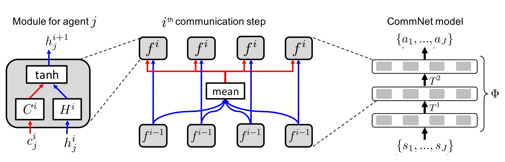
Figure 1: An overview of CommNet Model

CommNet alternates computation and communication so agents can share information. Left: The per-agent module for agent \(j\): the block \(f^i\) receives \(H^i_j\) (blue) and \(C^i_j\) (red), concatenates them, applies a nonlinearity (e.g., tanh), and outputs \(h^{i+1}_j\). Middle: One communication hop (\(i\)-th): part of each agent’s hidden state (blue) is passed forward; another part is sent onto the shared channel (red). The channel applies a mean aggregation and broadcasts the result back to every agent for the next hop. Right: The full CommNet: given inputs \({s_1,\dots,s_J}\), the network runs two communication hops (\(T^1,T^2\) here) and outputs actions \({a_1,\dots,a_J}\).

Model Extensions: Improvements for More Scenarios

To meet the needs of different tasks, CommNet has three important extensions:

Extension 1: Local Connectivity (Replacing Global Broadcast)

Not all agents need “full communication” — for example, in the traffic task, distant cars do not need to send signals to nearby cars. At this time, \(N(j)\) is used to represent the “communication neighbors” of agent \(j\) (e.g., other cars within a 3×3 range), and the communication vector is updated to the average of neighbors’ states:

\[ c_j^{i+1} = \frac{1}{|N(j)|} \sum_{j' \in N(j)} h_{j'}^{i+1}.(3) \]

Extension 2: Skip Connections (Retaining Initial Observations)

In some tasks, initial observations (e.g., agent IDs) are important. Therefore, \(h_j^0\) is also used as input to \(f^i\) to avoid losing key information during communication:

\[ h_j^{i+1} = f^i(h_j^i, c_j^i, h_j^0).(4) \]

Extension 3: Temporal Recurrence (Handling Dynamic Processes)

For multi-steps task (e.g., combat tasks with multiple rounds), the model is modified to RNN/LSTM, allowing hidden states to be passed across time steps to remember previous communication history:

\[ h_j^t = f^t(h_j^{t-1}, c_j^t) \]

where \(t\) is the time step, and actions are sampled at each time step.

Core Properties of CommNet

These designs give CommNet advantages not found in traditional models:

Property 1: Permutation Invariance

The order of agents does not affect the result. Since the communication vector is the “average of other agents’ states,” the T matrix (overall weight matrix for hidden state updates) is block-symmetric. No matter how the order of agents changes, the final action distribution remains unchanged — this is crucial for dynamically added agents.

Property 2: Dynamic Agent Adaptation

Due to the normalization factor of the communication vector being \(J-1\) (or \(|N(j)|\)), the size of the T matrix dynamically adjusts with the number of agents \(J\). It can handle scenarios where “agents join/leave” without retraining (e.g., more or fewer cars at a traffic intersection).

Property 3: Differentiable Continuous Communication

Communication vectors are continuous values, so the entire model can be trained through backpropagation — supporting both supervised learning (e.g., the “pull levers in order of ID” label for the lever-pulling task) and reinforcement learning (e.g., the “reduce collisions” reward for the traffic task). It is more flexible than discrete communication (which requires additional RL training).

Algorithm Design: Training Methods and Baseline Comparison

CommNet’s training is divided into two methods based on whether the task has “supervisory signals,” and it is compared with three classic baselines to highlight its advantages.

Two Training Methods

Supervised Learning

If each action has a correct label (e.g., in the lever-pulling task, “agents pull different levers in order of ID” is the correct solution), training is directly performed using cross-entropy loss:

\[ \mathcal{L} = -\sum_{j=1}^J \log q(h_j^K | a_j^*) \]

where \(a_j^*\) is the correct action.

Reinforcement Learning Training

If there are no supervisory signals (e.g., in the traffic task, it is unknown “when to brake” correctly), policy gradient + baseline is used for training.

Denote the states in an episode by \(s(1), ..., s(T)\), and the actions taken at each of those states as \(a(1), ..., a(T)\), where T is the length of the episode. The baseline is a scalar function of the states b(s, θ), computed via an extra head on the model producing the action probabilities. Beside maximizing the expected reward with policy gradient, the models are also trained to minimize the distance between the baseline value and actual reward. Thus after finishing an episode, we update the model parameters \(\theta\) by

\[ \Delta\theta=\sum_{t=1}^T\left[\frac{\partial\log p(a(t)|s(t),\theta)}{\partial\theta}\left(\sum_{i=t}^Tr(i)-b(s(t),\theta)\right)-\alpha\frac{\partial}{\partial\theta}\left(\sum_{i=t}^Tr(i)-b(s(t),\theta)\right)^2\right] \]

where \(a(t)\) is the concatenation of \(a_1(t), a_2(t), ..., a_J(t)\), \(s(t)\) is the concatenation of \(s_1(t), s_2(t), ..., s_J(t)\) \(b(s(t), \theta)\) is the state value baseline (reducing variance), and \(\alpha\) is the balance term (set to 0.03 in the paper).

Readers can see the supplementary material for details.

Baseline Models: What Makes CommNet Better?

The paper compares three mainstream baselines, and the results prove CommNet’s advantages:

Baseline Model	Core Logic	Drawbacks
Independent Controller	Each agent uses a separate Q-network without communication	Unable to collaborate (e.g., agents compete for levers in the lever-pulling task)
Fully Connected Model	Concatenates observations of all agents and uses a fully connected MLP to output actions	Fixed number of agents (retraining required when changing \(J\)) and order-sensitive
Discrete Communication	Agents send discrete symbols (e.g., 0/1), and the meaning of symbols is trained via RL	Communication signals are non-differentiable, unstable training, and performance is worse than continuous communication

Detailed Parameter Optimization Processes for CommNet

Feature : Global Unified Network + Shared Parameters

1. Parameter Initialization

Observation Preprocessing: Concatenate the local observations \(s_j\) of \(J\) agents into a global observation vector \(\pmb{s} = [s_1, s_2, ..., s_J]\). Convert this vector into initial hidden states \(h_j^0 = r(s_j)\) using an encoder \(r(\cdot)\), with encoder parameters shared among all agents.

Network Parameter Initialization: Initialize shared parameters, including:

• Hidden state update weights \(H^i\) and \(C^i\) (there are \(K\) communication rounds, with one set of \(H^i, C^i\) for each round);

• Decoder parameters \(q(\cdot)\);

2. Training Loop Phase

Forward Propagation: Global Observation → Communication → Action Output (The details have been shown in the part of Basic Communication Model).

Construction of Global Objective Function: Select either supervised learning or reinforcement learning (RL) objectives based on the task type and these formulas have been shown in the content of Two Training Methods.

Backward Propagation and Parameter Update

• Step 1: Gradient Calculation: Perform backward propagation along the path “decoder → communication layer → encoder”

• Step 2: Shared Parameter Update: Update all shared parameters.

Run CommNet in XuanCe

Before running CommNet in XuanCe, you need to prepare a conda environment and install xuancefollowing the installation steps.

Run Build-in Demos

After completing the installation, you can open a Python console and run CommNet directly using the following commands:

import xuance
runner = xuance.get_runner(algo='commnet',
                           env='mpe',  # Choices: mpe, sc2
                           env_id='simple_spread_v3',  # Choices: simple_spread_v3, etc
                           )
runner.run()

Run With Self-defined Configs

If you want to run CommNet with different configurations, you can build a new .yaml file, e.g., my_config.yaml. Then, run the CommNet by the following code block:

import xuance as xp
runner = xp.get_runner(algo='commnet',
                       env='mpe',  # Choices: mpe, sc2
                       env_id='simple_spread_v3',  # Choices: simple_spread_v3, etc
                       config_path="my_config.yaml",  # The path of my_config.yaml file should be correct.
                       )
runner.run()  # Or runner.benchmark()

To learn more about the configurations, please visit the tutorial of configs.

Run With Custom Environment

If you would like to run XuanCe’s CommNet in your own environment that was not included in XuanCe, you need to define the new environment following the steps in New Environment Tutorial. Then, prepapre the configuration file commnet_myenv.yaml.

After that, you can run CommNet in your own environment with the following code:

import argparse
from xuance.common import load_yaml
from xuance.environment import REGISTRY_ENV
from xuance.environment import make_envs
from xuance.torch.agents import CommNet_Agents

configs_dict = load_yaml(file_dir="commnet_myenv.yaml")
configs = argparse.Namespace(**configs_dict)
REGISTRY_ENV[configs.env_name] = MyNewEnv

envs = make_envs(configs)  # Make parallel environments.
Agent = CommNet_Agents(config=configs, envs=envs)  # Create CommNet agents from XuanCe.
Agent.train(configs.running_steps // configs.parallels)  # Train the model for numerous steps.
Agent.save_model("final_train_model.pth")  # Save the model to model_dir.
Agent.finish()  # Finish the training.

Citation

@article{sukhbaatar2016learning,
  title={Learning multiagent communication with backpropagation},
  author={Sukhbaatar, Sainbayar and Fergus, Rob and others},
  journal={Advances in neural information processing systems},
  volume={29},
  year={2016}
}