Deep Coordination Graphs (DCG)¶

Paper Link: https://proceedings.mlr.press/v119/boehmer20a/boehmer20a.pdf.

Cooperative multi-agent reinforcement learning (MARL) faces the curse of dimensionality: the joint action space grows exponentially with the number of agents. For example, 8 agents with 6 discrete actions each yield over a million joint actions. To cope, many MARL methods assume value factorization, where the centralized Q-function is decomposed into simpler components (for example, one per agent). The simplest factorization is fully decentralized: each agent has a utility function dependent only on its own action (as in VDN). While a sum of independent utilities can represent some optimal policies, this decomposition often fails when coordinated actions have significantly different value than uncoordinated ones. In particular, a well-known pathology is relative overgeneralization: during learning, an agent seeing other agents act randomly may undervalue a coordinated action, causing the joint optimal policy to be missed. In short, simple value decompositions (like VDN and QMIX) can lack the representational capacity to distinguish highly-coordinated joint actions, preventing learning of the true optimum.

../../../_images/DCG_value_factorization.png — Figure 1: Value factorization examples (VDN vs DCG vs QTRAN)¶

Figure 1 illustrates different factorization architectures for 3 agents: (a) VDN (independent utilities), (b) DCG (pairwise payoffs), (c) QTRAN (no factorization). This figure is from the DCG paper (Figure 1).

This table lists some general features about DCG algorithm:

Features of DCG	Values	Description
Fully Decentralized	❌	Agents communicate via message passing in coordination graphs, not fully decentralized without interaction.
Fully Centralized	❌	No central controller; decisions are made decentrally based on local interactions and message passing.
Centralized Training with Decentralized Execution (CTDE)	✅	Uses centralized information (e.g., agents’ histories, graph topology) during training and executes decentrally with message passing.
On-policy	❌	Adopts off-policy learning with experience replay (similar to DQN).
Off-policy	✅	The evaluation policy differs from the target policy, leveraging experience replay for sample efficiency.
Model-free	✅	Learns directly from interaction without relying on an environment dynamics model.
Model-based	❌	Does not require an environment model for policy training.
Discrete Action	✅	Designed to handle discrete action spaces, with low-rank approximation for scalability.
Continuous Action	❌	Primarily tailored for discrete action spaces; continuous action support is not a core feature.

1. Challenges in Cooperative MARL¶

The core challenge in cooperative MARL is scaling with joint action size. As the number of agents n grows, the joint action space |A₁×…×Aₙ| becomes prohibitively large. Without structure, estimating a centralized Q-function over this space is intractable. Simple decentralization, where each agent maximizes only a local utility function, gives tractable optimization but often misses necessary coordination: such factorizations can represent at least one optimal deterministic policy, but may not learn it in practice due to game-theoretic issues like relative overgeneralization. Even advanced factorizations like QMIX, which allow the central Q to be a monotonic mixture of per-agent utilities, cannot represent all possible value landscapes (the monotonicity constraint can preclude representing some optimal joint values). Thus, limited representational capacity and coordination difficulty are key problems in MARL. DCG was developed to address these by introducing more flexible factorization while retaining tractable learning and execution.

2. Limitations of VDN and QMIX¶

Value Decomposition Networks (VDN) and QMIX are popular MARL methods that impose specific factorizations on the joint Q-function. VDN simply sums individual agent utilities:

\[ Q_{VDN}(s,\mathbf{a}) = \sum_{i=1}^n f_i(a_i \mid \tau^i) \]

where each agent i has a utility $f_i$ depending on its local observation history $\tau^i$. In VDN, each agent can choose its action by independently maximizing $f_i$, which is computationally efficient. However, this representation is too restrictive: it assumes that the best joint action is obtained by each agent taking its individually best action. In many tasks, the best joint outcome requires sacrificing immediate individual utility for the sake of coordination. If the function class $f_i$ cannot capture the extra reward from coordination, the learning algorithm cannot distinguish a high-value coordinated action from uncoordinated ones, and will not converge to the true optimal policy.

QMIX generalizes VDN by introducing a mixing network $ϕ$ that takes all agent utilities as inputs and produces the joint Q-value:

\[ Q_{QMIX}(s,\mathbf{a}) = ϕ\Big(s,\; f_1(a_1 \mid \tau^1),\ldots,f_n(a_n \mid \tau^n)\Big)\,. \]

Crucially, $ϕ$ is constrained to be monotonic in each utility input. This monotonicity ensures that maximizing individual $f_i$ still yields the best joint action. QMIX can represent a larger class of value functions than VDN, especially by using the global state $s$ as input to $ϕ$, but it cannot capture non-monotonic interactions. In practice, tasks with hard coordination often involve value functions that are non-monotonic in individual utilities, so QMIX (and VDN) fail to learn the optimal policy. In summary, although VDN/QMIX are tractable, their restrictive factorizations lead to failure modes (like relative overgeneralization) in genuinely cooperative tasks.

DCG without edges (VDN) has to fail eventually (p < −1).

../../../_images/DCG-Performance-Comparison.png — Figure 2: Performance Comparison in Overgeneralization Task¶

This figure 2 shows how different models perform in the relative overgeneralization task where 8 agents hunt 8 prey. The fully connected DCG is able to represent the value of joint actions, leading to better performance for larger p, while DCG without edges (VDN) fails for lower values of p. CG without parameter sharing learns very slowly due to sample inefficiency.

3. Deep Coordination Graphs (DCG): Graphical Factorization and Message Passing¶

DCG overcomes these limitations by using a coordination graph (CG) to define the factorization of the joint Q-function. A coordination graph is an undirected graph $\mathcal{G}=\langle\mathcal{V},\mathcal{E}\rangle$ where each vertex corresponds to an agent and each edge $\{i,j\}\in \mathcal{E}$ indicates a pairwise payoff function between agents $i$ and $j$. In DCG, the Q-function is factored into per-agent utilities and pairwise payoffs along the edges of the graph:

\[ Q^{\mathrm{CG}}(s_{t},\boldsymbol{a}):=\frac{1}{|\mathcal{V}|}\sum_{v^{i}\in\mathcal{V}}f^{i}(a^{i}|s_{t})+\frac{1}{|\mathcal{E}|}\sum_{\{i,j\}\in\mathcal{E}}f^{ij}(a^{i},a^{j}|s_{t}). \]

Here each utility $f_i$ depends on agent $i$’s action $a_i$ (and possibly its observation history), and each payoff $f_{ij}$ depends on the joint actions of agents $i$ and $j$ (and optionally on the state). The normalization factors $1/|\mathcal{V}|$ and $1/|\mathcal{E}|$ are optional scaling; the core idea is that the joint value is the average of individual and pairwise contributions. When $\mathcal{E}=\emptyset$, this reduces to VDN. Adding each edge adds capacity: each pairwise payoff can model a coordinating effect that independent utilities cannot. In effect, DCG learns a richer class of value functions that include pairwise agent interactions.

Once the joint Q-function is factorized by a CG, the optimal joint action (or greedy action) cannot in general be found by each agent separately. Instead, DCG uses max-sum message passing (a form of belief propagation) on the coordination graph to compute (approximately) the joint argmax of $Q_{DCG}$. In a tree-structured graph, max-sum is guaranteed to converge to the true maximum. Concretely, each edge $(i,j)$ carries a message vector $\mu_{ij}(a_j)$ representing the influence of agent $i$ on agent $j$’s action value. Messages are iteratively updated by:

$\mu_{t}^{ij}(a^{j}) \leftarrow \max_{a^{i}}\left\{\frac{1}{|\mathcal{V}|}f^{i}(a^{i}\mid s_{t}) + \frac{1}{|\mathcal{E}|}f^{ij}(a^{i},a^{j}\mid s_{t}) + \sum_{k:(k,i)\in\mathcal{E}}\mu_{t}^{ki}(a^{i}) - \mu_{t}^{ji}(a^{i})\right\}$

where the sum is over incoming messages to $i$ from its other neighbors, and $-\mu_{ji}$ avoids double-counting. After sufficient iterations (denote $t$ the final step), each agent $i$ chooses the action that maximizes its local estimate of the joint Q-value:

$a_{*}^{i} := \arg\max_{a^{i}}\left\{\frac{1}{|\mathcal{V}|}f^{i}(a^{i}\mid s_{t}) + \sum_{k:(k,i)\in\mathcal{E}}\mu_{t}^{ki}(a^{i})\right\}$

This scheme finds the joint greedy action $\mathbf{a}^*$ that (approximately) maximizes $Q_{DCG}(s,\mathbf{a})$. In acyclic CGs, the max-sum updates converge to the exact optimum. In cyclic graphs, DCG uses heuristic message normalization (subtracting a mean term) to improve convergence. The key advantage of DCG is that the representation is powerful enough to capture coordination, yet inference remains local. Compared to a fully centralized Q, DCG’s message passing takes $O(km(n+m)|E|)$ time per decision (for $k$ iterations, $n$ agents, $m$ actions each) which is tractable for sparse graphs. Importantly, DCG employs parameter sharing: all payoff networks $f_{ij}$ share the same weights (conditioned on agent IDs), and all utilities $f_i$ share weights. This sharing, along with optional low-rank factorization of payoffs, dramatically improves sample efficiency.

4. Core Q-Function and Design Principles of DCG¶

1. Core Q-Function of DCG¶

DCG achieves value decomposition based on a coordination graph, with its core joint Q-function formulated as follows:

\[ q_{\theta\phi\psi}^{\mathrm{DCG}}(\boldsymbol{\tau}_{t},\boldsymbol{a}) := \frac{1}{|\mathcal{V}|}\sum_{i=1}^{n}\overbrace{f_{\theta}^{v}(a^{i}|\boldsymbol{h}_{t}^{i})}^{f_{i,a^{i}}^{\mathrm{V}}} + \frac{1}{2|\mathcal{E}|}\sum_{\{i,j\}\in\mathcal{E}}\underbrace{f_{\phi}^{e}(a^{i},a^{j}|\boldsymbol{h}_{t}^{i},\boldsymbol{h}_{t}^{j})+f_{\phi}^{e}(a^{j},a^{i}|\boldsymbol{h}_{t}^{j},\boldsymbol{h}_{t}^{i})}_{f_{\{i,j\},a^{i},a^{j}}^{\mathrm{E}}} \]

Where:

$q^{DCG}(a|\tau_t)$ denotes the expected discounted sum of rewards for executing the joint action $a$ under the agents’ history $\tau_t$;
$|\mathcal{V}|$ is the total number of agents (number of vertices in the coordination graph), and $|\mathcal{E}|$ is the total number of agent pairs (number of edges in the coordination graph);
$f_\theta^v(a^i|h_t^i)$ is the individual utility function of agent $i$ (parameterized by $\theta$, with input as the RNN hidden state $h_t^i$);
$f_\phi^e(a^i,a^j|h_t^i,h_t^j)$ is the pairwise payoff function between agent $i$ and agent $j$ (parameterized by $\phi$, with inputs as the RNN hidden states $h_t^i$ and $h_t^j$ of the two agents).

2. Core Design Principles of DCG¶

Payoff functions depend only on local information (the histories $\tau_t^i$ and $\tau_t^j$ of agents $i$ and $j$);
All payoff/utility functions share parameters (via a common RNN);
Low-rank approximation is applied to payoff matrices;
Support for cross-graph generalization (permutation invariance).

5. DCG Algorithms and Pseudocode¶

Below we outline the three key computational procedures in DCG.

5.1. Annotating the Coordination Graph (Utility and Payoff Computation)¶

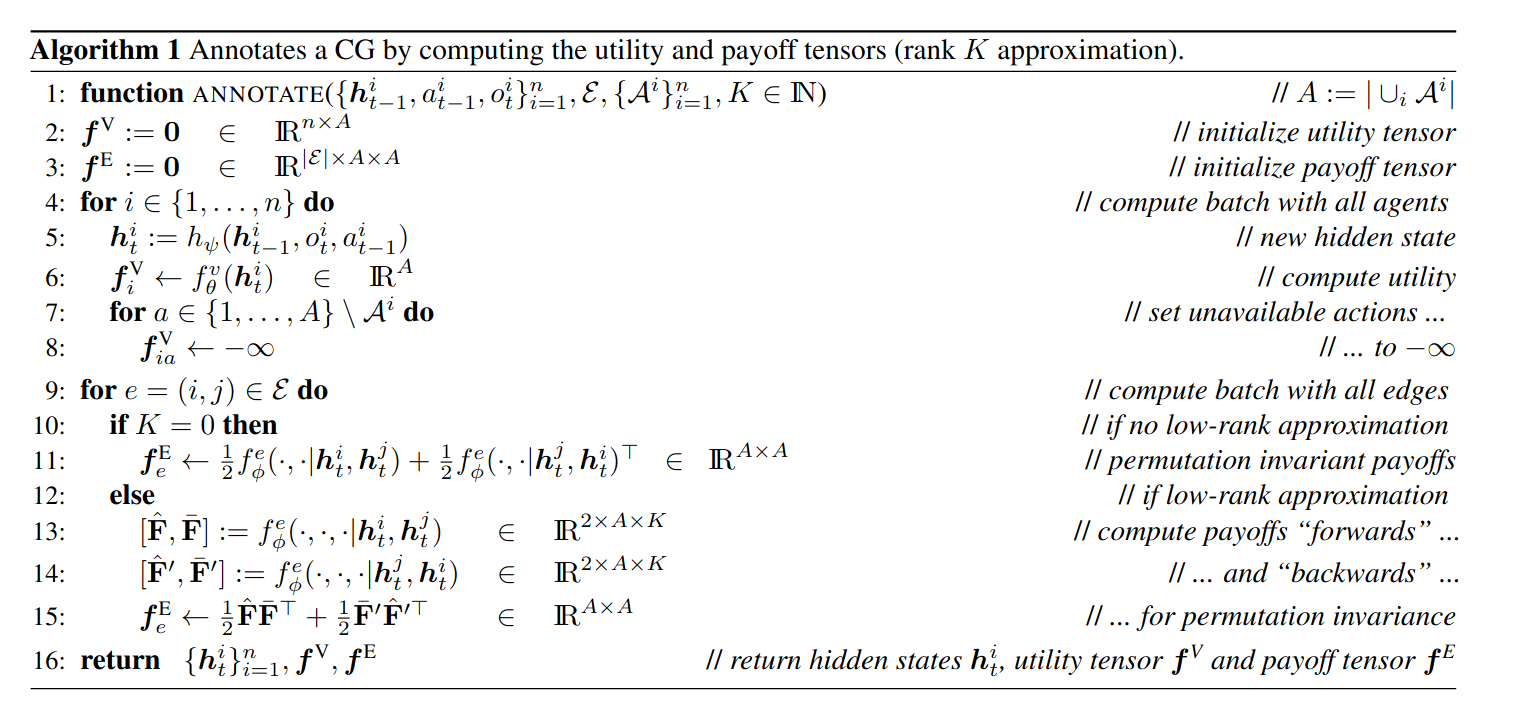
../../../_images/pseucode-DCG-1.png — pseudocode 1: Annotating the Coordination Graph pseudocode¶

This pseudocode computes the utility and payoff tensors for each agent and pair of agents. It updates the hidden states of each agent based on its previous state, observation, and action, and then computes the individual utilities and pairwise payoffs based on the coordination graph.

5.2. Q-value Computation¶

../../../_images/pseucode-DCG-2.png — pseudocode 2: Q-value Computation pseudocode¶

This pseudocode computes the joint Q-value by combining the individual agent utilities and pairwise payoffs. The computed Q-values are used to evaluate the quality of the joint actions, which is crucial for selecting optimal actions in the DCG framework.

5.3. Greedy Action Selection with Message Passing¶

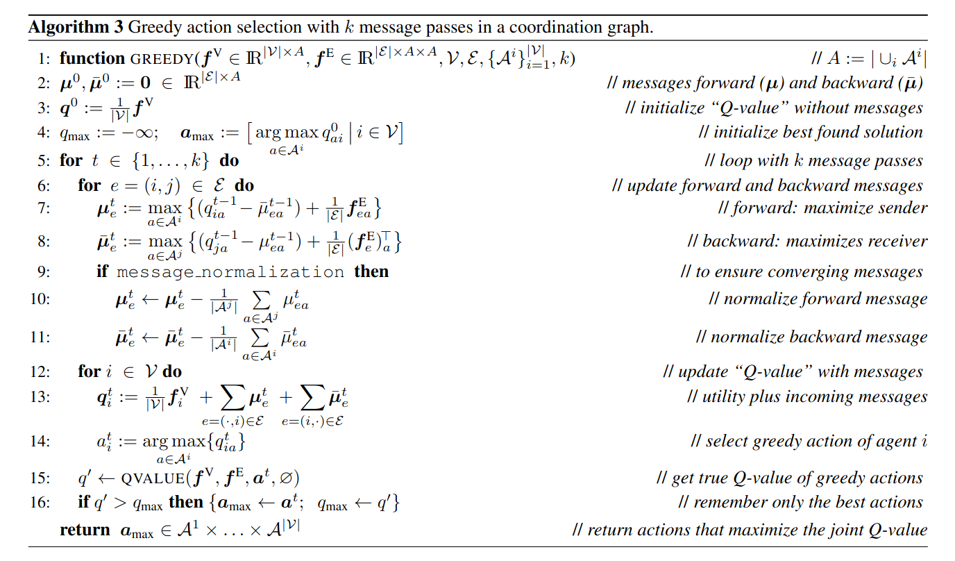
../../../_images/pseucode-DCG-3.png — pseudocode 3: Greedy Action Selection with Message Passing pseudocode¶

This pseudocode implements the greedy action selection using message passing on the coordination graph. The messages are iteratively updated and used by each agent to select the action that maximizes its contribution to the joint Q-value, ensuring coordinated decision-making in the DCG method.

Run DCG in XuanCe¶

Before running DCG in XuanCe, you need to prepare a conda environment and install xuance following the installation steps.

import xuance
# Create runner for DCG algorithm
runner = xuance.get_runner(algo='dcg',
                           env='sc2',  # Choices: sc2, mpe
                           env_id='3m',  # Choices: 3m, 2m_vs_1z, 8m, 1c3s5z, 2s3z, 25m, 5m_vs_6m, 8m_vs_9m, MMM2, etc.
                           )  # False for training, True for testing
runner.run()  # Start running (or runner.benchmark() for benchmarking)

Run With Self-defined Configs¶

If you want to run DCG with different configurations, you can build a new .yaml file, e.g., my_config.yaml. Then, run the DCG by the following code block:

import xuance as xp
# Create runner for DCG algorithm
runner = xp.get_runner(algo='DCG',
                       env='sc2',  # Choices: sc2, mpe
                       env_id='3m',  # Choices: 3m, 2m_vs_1z, 8m, 1c3s5z, 2s3z, 25m, 5m_vs_6m, 8m_vs_9m, MMM2, etc.
                       config_path="my_config.yaml",  # The path of my_config.yaml file should be correct.
                       )  # False for training, True for testing
runner.run()  # Start running (or runner.benchmark() for benchmarking)

To learn more about the configurations, please visit the tutorial of configs.

Run With Custom Environment¶

If you would like to run XuanCe’s DCG in your own environment that was not included in XuanCe, you need to define the new environment following the steps in New Environment Tutorial. Then, prepapre the configuration file dcg_myenv.yaml.

After that, you can run DCG in your own environment with the following code:

import argparse
from xuance.common import load_yaml
from xuance.environment import REGISTRY_MULTI_AGENT_ENV
from xuance.environment import make_envs
from xuance.torch.agents.multi_agent_rl.dcg_agents import DCG_Agents

configs_dict = load_yaml(file_dir="DCG_myenv.yaml")
configs = argparse.Namespace(**configs_dict)
REGISTRY_MULTI_AGENT_ENV[configs.env_name] = MyNewEnv

envs = make_envs(configs)  # Make parallel environments.
Agent = DCG_Agents(config=configs, envs=envs)  # Create a DCG agent from XuanCe.
Agent.train(configs.running_steps // configs.parallels)  # Train the model for numerous steps.
Agent.save_model("final_train_model.pth")  # Save the model to model_dir.
Agent.finish()  # Finish the training.

Citation¶

@InProceedings{pmlr-v119-boehmer20a,
  title = {Deep Coordination Graphs},
  author = {Boehmer, Wendelin and Kurin, Vitaly and Whiteson, Shimon},
  booktitle = {Proceedings of the 37th International Conference on Machine Learning},
  pages = {980--991},
  year = {2020},
  editor = {III, Hal Daumé and Singh, Aarti},
  volume = {119},
  series = {Proceedings of Machine Learning Research},
  month = {13--18 Jul},
  publisher = {PMLR},
  pdf = {http://proceedings.mlr.press/v119/boehmer20a/boehmer20a.pdf},
  url = {https://proceedings.mlr.press/v119/boehmer20a.html},
}