Q-Transformation (QTRAN)
Paper Link: http://proceedings.mlr.press/v97/son19a.html.
QTRAN is a value decomposition method proposed in Multi-Agent Reinforcement Learning (MARL) to overcome the structural limitations of classical algorithms. Unlike algorithms such as QMIX that rely on monotonicity constraints, QTRAN innovatively introduces a transformed joint action-value function, enabling it to represent a broader range of cooperative strategies. The algorithm demonstrates exceptional performance in non-monotonic tasks such as cooperative predation, significantly outperforming mainstream algorithms like QMIX and highlighting its strong potential for complex multi-agent collaboration.
This table lists some general features about QTRAN algorithm:
Features of QTRAN |
Values |
Description |
|---|---|---|
Fully Decentralized |
❌ |
There is no communication between agents. |
Fully Centralized |
❌ |
Agents send all information to the central controller, and the controller will make decisions for all agents. |
Centralized Training with Decentralized Execution (CTDE) |
✅ |
The central controller is used in training and abandoned in execution. |
On-policy |
❌ |
The evaluate policy is the same as the target policy. |
Off-policy |
✅ |
The evaluate policy is different from the target policy. |
Model-free |
✅ |
No need to prepare an environment dynamics model. |
Model-based |
❌ |
Need an environment model to train the policy. |
Discrete Action |
✅ |
Deal with discrete action space. |
Continuous Action |
❌ |
Deal with continuous action space. |
1. Research Background and Motivation
The previously introduced VDN, QMIX, and WQMIX algorithms are all value-based methods used in cooperative multi-agent reinforcement learning (MARL) tasks. These algorithms essentially aim to find distributed optimal policies that satisfy the relationship described by the following equation:
Here, \(Q_{jt}\) represents the joint action-value function, and \(Q_i\) denotes the value function of agent \(i\). In this paper, the authors define the relationship in Equation (1) as the IGM (Individual-Global-Max) condition.
To satisfy the IGM condition, VDN directly decomposes the value function into an “additive form”:
From Equation (2), it can be derived that\(\frac{\partial Q_{jt}(\boldsymbol{\tau}, \mathbf{u})}{\partial Q_i(\tau_i, u_i)} \equiv 1, \quad \forall i \in \mathcal{N}.\)which indicates that satisfying Equation (2) is sufficient to meet the IGM condition.
However, QMIX considered VDN’s approach too restrictive for effectively fitting many complex functions. Thus, QMIX proposed a more general monotonicity condition:
QMIX argues that satisfying Equation (3) is sufficient to meet the IGM condition.
Indeed, Equation (2) is a sufficient condition for Equation (3), but at the same time, Equation (3) is also a sufficient condition for Equation (1). In other words, neither is necessary for the IGM condition! Therefore, for some cooperative problems with non-monotonic returns, the function approximation capabilities of VDN and QMIX become limited—this aligns with the research motivation behind the WQMIX algorithm.
Thus, to address this issue, the authors propose the QTRAN algorithm and claim that it can decompose any decomposable task without being constrained by Equations (2) and (3) .
2. Algorithm Approach
The core idea of the authors is to map the original joint value function \(Q_{jt}(\boldsymbol{\tau}, \mathbf{u})\) to a new value function \(Q'_{jt}(\boldsymbol{\tau}, \mathbf{u})\), such that the optimal joint actions of these two functions are equivalent. This allows us to obtain individual value functions \([Q_i]\) by decomposing \(Q'_{jt}\), while also establishing the relationship between \(Q'_{jt}\) and \(Q_{jt}\) to ensure global optimality.
Clearly, such a mapping cannot be arbitrary. To guarantee global optimality, the authors first propose the conditions that the value function decomposition must satisfy.
2.1 Conditions for Value Function Factorization
Let \(\bar{u}_i = \arg \max_{u_i} Q_i(\tau_i, u_i)\) denote the optimal local action of agent \(i\); \(\bar{\mathbf{u}} = [\bar{u}_i]_{i=1}^N\) denote the joint optimal local action; \(\mathbf{Q} = [Q_i]_{i=1}^N \in \mathbb{R}^N\) denote the joint value function vector. The authors provide the following conclusion:
Theorem 1.
When \(Q_{jt}(\boldsymbol{\tau}, \mathbf{u})\) and \([Q_i(\tau_i, u_i)]_{i=1}^N\) satisfy the following relationship:
where \(V_{jt}(\boldsymbol{\tau}) = \max_{\mathbf{u}} Q_{jt}(\boldsymbol{\tau}, \mathbf{u}) - \sum_{i=1}^N Q_i(\tau_i, \bar{u}_i)\) , then the joint action-value function \(Q_{jt}(\boldsymbol{\tau}, \mathbf{u})\) can be decomposed into \([Q_i(\tau_i, u_i)]_{i=1}^N\).
Theorem 1 indicates that as long as the relationship in Equation (4) is satisfied, the IGM condition can be fulfilled. The following analysis explores the mathematical logic of this theorem to aid in-depth understanding (for detailed proof, please refer to the appendix in the original text).
Sufficiency:
We can rewrite the left-hand side of the \(Q_{jt}\) expression as:
Observe that when \(\mathbf{u} = \bar{\mathbf{u}}\), we have \(\max_{u_i} Q_i(\tau_i, u_i) - Q_i(\tau_i, u_i) = 0\). In this case, if \(\delta = 0\), it implies \(\max_{\mathbf{u}} Q_{jt}(\boldsymbol{\tau}, \mathbf{u}) - Q_{jt}(\boldsymbol{\tau}, \bar{\mathbf{u}}) = 0\). Therefore, the IGM condition is satisfied.
When \(\mathbf{u} \neq \bar{\mathbf{u}}\), if \(\delta \geq 0\), it means:
Thus, \(\max_{\mathbf{u}} Q_{jt}(\boldsymbol{\tau}, \mathbf{u}) \geq Q_{jt}(\boldsymbol{\tau}, \mathbf{u})\), meaning the optimum is not achieved. In other words, the global value function reaches its optimum only when \(\mathbf{u} = \bar{\mathbf{u}}\).
From this perspective, the condition is quite sufficient. However, is it necessary?
Necessity:
The authors indicate in the paper that under the affine transformation \(\phi(\mathbf{Q}) = {A} \cdot \mathbf{Q} + {B}\), Equation (4) is necessary. Here,
\({A} = [a_{ii}]\) is a diagonal matrix with all positive elements, and \({B} = [b_i]\) is a bias term.
This implies that as long as the IGM condition holds, there must exist an affine transformation \(\phi\) that, after appropriately stretching and scaling the decomposed value function vector \(\mathbf{Q}\) (replacing \(Q_i\) with \((a_{ii} \cdot Q_i + b_i)\)), satisfies the relationship in Equation (4).
Therefore, the authors state that Equation (4) is a necessary condition for IGM under affine transformation.
2.2 How to Map?
For the new value function \(Q_{jt}'\), the authors directly define it as:
(Wait , isn’t this just VDN? Don’t worry, let’s see how it differs from VDN.)
Because VDN’s decomposition is overly sufficient, there is a gap between it and the true \(Q_{jt}\). Therefore, based on the definition of \(V_{jt}(\boldsymbol{\tau})\) in Theorem 1, the authors propose using \(V_{jt}(\boldsymbol{\tau})\) to correct the error between \(Q_{jt}\) and \(Q_{jt}'\). This leads to:
In this way, we establish the relationship between \(Q_{jt}\) and \(Q_{jt}'\). Notice that \([Q_i]\) serves as the decomposition for both \(Q_{jt}\) and \(Q_{jt}'\), sohe optimal actions selected using them are equivalent.
If we directly fit \(Q_{jt}'\) as the value function, it would be the same as the VDN algorithm — the key difference lies in the relationship described in Equation (6). Therefore, learning \(V_{jt}\) becomes particularly crucial.
3. Algorithm Design
3.1 Structural Framework
Based on the above analysis, there are at least three components that need to be learned: \(Q_i\), \(Q_{jt}\), and \(V_{jt}\). Therefore, the QTRAN algorithm framework correspondingly includes the following three important modules:
Individual Action-Value Network: \(f_q : (\tau_i, u_i) \mapsto Q_i\);
Joint Action-Value Network: \(f_r : (\boldsymbol{\tau} ,\mathbf{u}) \mapsto Q_{jt}\);
State-Value Network: \(f_v : \boldsymbol{\tau} \mapsto V_{jt}\).
Algorithm Block Diagram:

In the diagram, the design of the individual agent network \(f_q\) is similar to that of VDN and QMIX. We primarily focus on the design of \(f_r\) and \(f_v\):
When updating this network, the individual agent network is used to compute the traversal of the next actions, rather than performing the \(\arg\max\) operation over the entire joint action space \(\mathcal{U}^N\).
The \(f_r\) network shares parameters with the \(f_q\) network in the earlier layers.
The state-value network \(f_v\) functions similarly to the \(V(s)\) in a dueling network. Additionally, \(f_v\) also shares parameters with the \(f_q\) network in the earlier layers.
3.2 Loss Function
Since QTRAN has two training objectives: \(Q_{jt}\) and \(V_{jt}\), the loss function is designed as follows:
\(L_{td}\) is used to fit \(Q_{jt}\); \(L_{opt}\) and \(L_{nopt}\) are used to fit \(V_{jt}\). They are defined as:
Here, \(\theta^-\) represents the target network parameters. \(L_{opt}\) ensures that Equation (4a) holds, while \(L_{nopt}\) ensures that Equation (4b) holds.
3.3 Variant of QTRAN: QTRAN-alt
The QTRAN method described earlier is referred to by the authors as QTRAN-base. They argue that the condition in Equation (4b), which applies to all actions, is inefficient and can negatively impact the algorithm’s stability and convergence speed. Therefore, they revised the condition (4b) in Theorem 1 and proposed Theorem 2:
Theorem 2. When \(\mathbf{u} \neq \bar{\mathbf{u}}\), replacing condition (4b) in Theorem 1 with the following equation still ensures the validity of Theorem 1:
where \(\mathbf{u}_{-i} = (u_1, \ldots, u_{i-1}, u_{i+1}, \ldots, u_N)\).
The proof of Theorem 2 can likewise be found in the appendix. Equation (7) is stricter than Equation (4b) because it forces \(Q'_{jt}\) to track the updates of the true \(Q_{jt}\) . The algorithm based on Theorem 2 is called QTRAN-alt, where “alt” stands for “alternative.”
To facilitate the computation of the min function in Equation (7), the authors draw inspiration from the counterfactual baseline concept in the COMA algorithm and propose a counterfactual joint network. Ultimately,
This allows the \(L_{nopt}\) loss to be rewritten as:
where,
In QTRAN-alt, the computation of \(L_{nopt\text{-}min}\) only requires traversing the local action space of individual agents. However, similar to QTRAN-base, both \(L_{td}\) and \(L_{opt}\) still require traversing the joint action space of all agents.
3.4 Algorithm Pseudocode
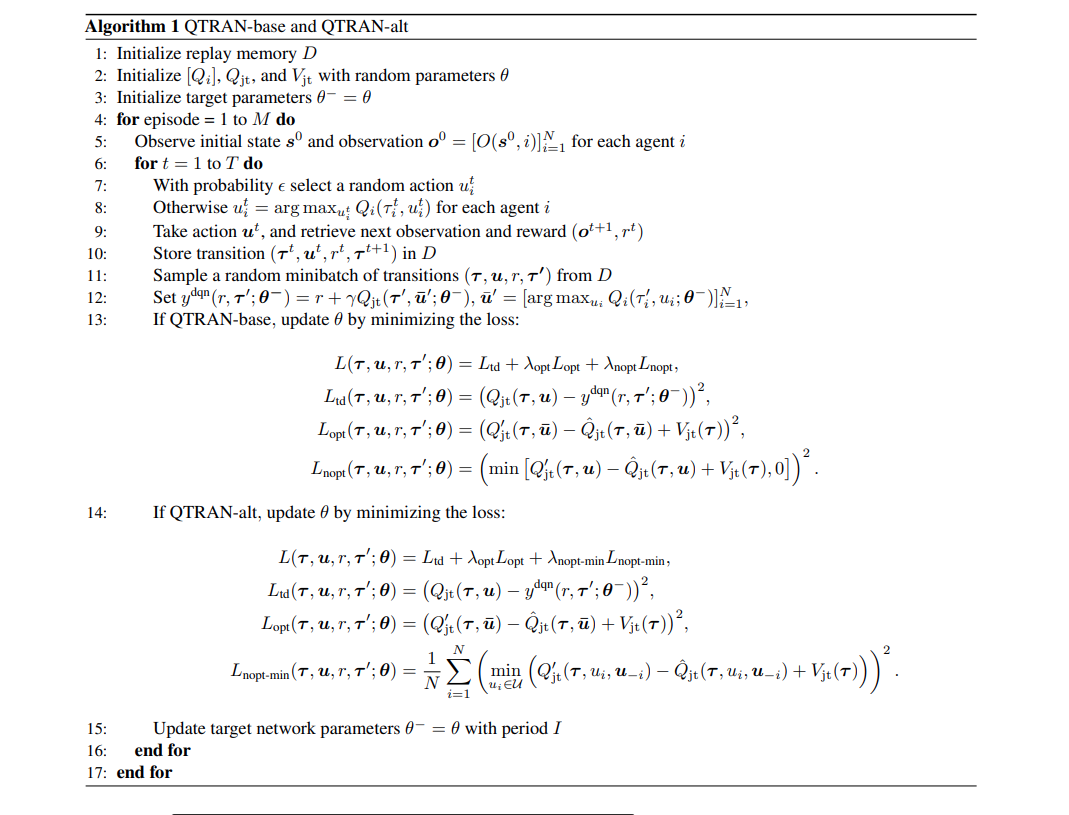
3.5 Case Study: Single-state Matrix Game
To demonstrate the performance of the two QTRAN algorithms, the authors first present a simple single-step matrix game case. The table below shows the corresponding payoff matrix and the Q-values learned by various algorithms. Here, A, B, and C represent the actions available to each agent. (For details on how the learning process works, please refer to the description in the original paper.)

Table 1. Single-step Matrix Game Model, bold represents the optimal Q-values.
In this case, the payoff matrix is non-monotonic. As a result, both the VDN algorithm and the QMIX algorithm converge to local optima, while QTRAN can almost perfectly approximate the true payoff matrix. From Table 1, we can draw at least the following conclusions:
The value function obtained by the VDN algorithm deviates the most from the true values (Table e);
QMIX fails to accurately approximate the Q-values for action group AA and can only reach a local optimum (Table f);
By effectively compensating for the error between VDN and the true Q-values (Table d), QTRAN learns a decomposed value function that achieves the global optimum (Tables b and c), thereby satisfying the IGM condition.
Due to the limited number of actions in this case, the differences between the two QTRAN variants are not apparent. To address this, the authors conducted a comparative experiment between QTRAN-base and QTRAN-alt on a matrix game with 21 actions. The results are as follows:

Figure 2. Performance comparison of QTRAN-base and QTRAN-alt algorithms.
In the figure, the horizontal and vertical coordinates represent the actions selected by the two agents, respectively, and the color depth indicates the magnitude of the Q-values. From the figure, it is relatively clear that for the learning of \(Q'_{jt}\), QTRAN-base fits the Q-values corresponding to the optimal actions well, but exhibits larger errors for non-optimal actions. In contrast, QTRAN-alt achieves more accurate Q-value approximations for both optimal and non-optimal actions.
Run QTRAN in XuanCe
Before running QTRAN in XuanCe, you need to prepare a conda environment and install xuance following
the installation steps.
Run Build-in Demos
After completing the installation, you can open a Python console and run QTRAN directly using the following commands:
import xuance
runner = xuance.get_runner(algo='qtran',
                           env='sc2',  # Choices: mpe.
                           env_id='8m', # Choices: 1c3sc5, 3m, MMM2, 25m.
                           )
runner.run()  # Or runner.benchmark()
Run With Self-defined Configs
If you want to run QTRAN with different configurations, you can build a new .yaml file, e.g., my_config.yaml.
Then, run the QTRAN by the following code block:
import xuance
runner = xuance.get_runner(algo='qtran',
                       env='sc2',  # Choices: mpe.
                       env_id='8m', # Choices: 1c3sc5, 3m, MMM2, 25m.
                       config_path="my_config.yaml",  # The path of my_config.yaml file should be correct.
                       )
runner.run()  # Or runner.benchmark()
To learn more about the configurations, please visit the tutorial of configs.
Run With Custom Environment
If you would like to run XuanCe’s QTRAN in your own environment that was not included in XuanCe,
you need to define the new environment following the steps in
New Environment Tutorial.
Then, prepapre the configuration file
qtran_myenv.yaml.
After that, you can run QTRN in your own environment with the following code:
import argparse
from xuance.common import load_yaml
from xuance.environment import REGISTRY_MULTI_AGENT_ENV
from xuance.environment import make_envs
from xuance.torch.agents.multi_agent_rl.qtran_agents import QTRAN_Agents

configs_dict = load_yaml(file_dir="qtran_myenv.yaml")
configs = argparse.Namespace(**configs_dict)
REGISTRY_MULTI_AGENT_ENV[configs.env_name] = MyNewEnv

envs = make_envs(configs)  # Make parallel environments.
Agent = QTRAN_Agents(config=configs, envs=envs)  # Create a VDN agent from XuanCe.
Agent.train(configs.running_steps // configs.parallels)  # Train the model for numerous steps.
Agent.save_model("final_train_model.pth")  # Save the model to model_dir.
Agent.finish()  # Finish the training.
Citation
@inproceedings{son2019qtran,
  title={QTRAN: Learning to Factorize with Transformation for Cooperative Multi-Agent Reinforcement Learning},
  author={Son, Kyunghwan and Kim, Daewoo and Kang, Wan Ju and Hostallero, David Earl and Yi, Yung},
  booktitle={International Conference on Machine Learning},
  pages={5887--5896},
  year={2019},
  organization={PMLR}
}