Weighted Q-Mixing Networks (WQMIX)

Paper Link: https://proceedings.neurips.cc/paper_files/paper/2020/file/73a427badebe0e32caa2e1fc7530b7f3-Paper.pdf.

Today, we continue to introduce the Weighted QMIX (WQMIX) algorithm — a value-based multi-agent reinforcement learning (MARL) algorithm. As its name suggests, WQMIX is an improved version of QMIX. If you are not familiar with the QMIX algorithm, it is recommended to first refer to the document that analyzes the QMIX algorithm.

The WQMIX algorithm was also developed by members of the Whiteson Research Lab at the University of Oxford and was published at NeurIPS 2020.

This table lists some general features about WQMIX algorithm:

Features of WQMIX	Values	Description
Fully Decentralized	❌	There is no communication between agents.
Fully Centralized	❌	Agents send all information to the central controller and the controller will make decisions for all agents.
Centralized Training With Decentralized Execution (CTDE)	✅	The central controller is used in training and abandonded in execution.
On-policy	❌	The evaluate policy is the same as the target policy.
Off-policy	✅	The evaluate policy is different from the target policy.
Model-free	✅	No need to prepare an environment dynamics model.
Model-based	❌	Need an environment model to train the policy.
Discrete Action	✅	Deal with discrete action space.
Continuous Action	❌	Deal with continuous action space.

Research Background and Motivation

In MARL environments for cooperative tasks, multiple agents share a single reward signal. This often leads to the problems of “lazy agents” and “credit assignment”. To address these issues, the VDN algorithm proposes decomposing the system’s total value function using a simple summation: \(Q_{tot}(\boldsymbol{\tau},\boldsymbol{u})=\sum_{i=1}^nQ_i(\tau_i,u_i)\). This value function factorization method is straightforward, but its over-compliance with the “monotonicity” constraint severely limits its ability to approximate nonlinear functions. To overcome this limitation, the QMIX algorithm was proposed. It uses a Mixing Network to fit \(Q_{tot}^*\), significantly enhancing the network’s nonlinear function approximation capability while satisfying the “monotonicity” requirement for decentralized policies.

However, as noted in our previous analysis of QMIX, the monotonicity constraint satisfied by QMIX is a sufficient but not necessary condition. This means there exist scenarios where QMIX cannot accurately fit the value function. For example, when agents’ actions influence each other (i.e., an agent’s decision must consider the actions of other agents), QMIX fails to account for such interdependencies. As a result, QMIX’s function representation capability remains limited.

Thus, the primary goal of this research is to further break free from the constraints on QMIX’s function representation capability.

QMIX Operator: Definition and Properties

Definition of the QMIX Operator: \(\mathcal{T}_{\mathrm{Qmix}}^*\)

To simplify understanding and analysis, the authors assume that all agents observe the global state \(s\) and use Q-tables for analysis.

First, they define the function space to which \(Q_{tot}\) belongs:

\[ \mathcal{Q}^{mix}=\{Q_{tot}|Q_{tot}(s,\boldsymbol{u})=f_{s}(Q_{1}(s,u_{1}),\cdots,Q_{n}(s,u_{n})),\frac{\partial f_{s}}{\partial Q_{a}}\geq0,Q_{a}(s,u)\in\mathbb{R}\} \]

As analyzed in the QMIX’s document, the design of the QMIX algorithm ensures that the network can approximate any function in \(\mathcal{Q}^{mix}\) with arbitrary precision. QMIX can be formulated as the following optimization problem:

\[ \arg\min_{q\in\mathcal{Q}^{mix}}\sum_{\boldsymbol{u}\in\boldsymbol{U}}(\mathcal{T}^*Q_{tot}(s,\boldsymbol{u})-q(s,\boldsymbol{u}))^2,\forall s\in S.(1) \]

Here, \(\mathcal{T}^*\) denotes the Bellman optimal operator:

\[ \mathcal{T}^*Q(s,\boldsymbol{u}):=\mathbb{E}[r+\gamma\max_{\boldsymbol{u}^{\prime}}Q(s^{\prime},\boldsymbol{u}^{\prime})].(2) \]

The authors define the optimization problem in Equation\(`(1)`\) as the QMIX operator, denoted \(\mathcal{T}_{\mathrm{Qmix}}^*\).

It can be viewed as the composition of two operators:

\[ \mathcal{T}_{\mathrm{Qmix}}^*=\Pi_{\mathrm{Qmix}}\mathcal{T}^*.(3) \]

where \(\Pi_{\mathrm{Qmix}}\) is defined as:

\[ \Pi_{\mathrm{Qmix}}Q:=\arg\min_{q\in\mathcal{Q}^{mix}}\sum_{\boldsymbol{u}\in \boldsymbol{U}}(Q(s,\boldsymbol{u})-q(s,\boldsymbol{u}))^2.(4) \]

Geometrically, \(\Pi_{\mathrm{Qmix}}Q\) represents the point in the function space \(\mathcal{Q}^{mix}\) that is closest to the function \(Q\), measured by the L2 norm.

Properties of the \(\mathcal{T}_{\mathrm{Qmix}}^*\) Operator

Since the optimization in Equation\(`(1)`\) is performed within the \(`\mathcal{Q}^{mix}`\) space, QMIX may fail to find the fixed point of \(`\mathcal{T}^*`\) in some cases. Instead, it can only find a suboptimal solution in \(`\mathcal{Q}^{mix}`\) that is closest to the fixed point. Consequently, the optimization result of Equation\(`(1)`\) may not be unique, and \(`\mathcal{T}_{\mathrm{Qmix}}^*`\) will randomly return a \(`q`\)-function as the final solution.

Property 1: \(\mathcal{T}_{\mathrm{Qmix}}^*\) is not a contraction mapping.

Those familiar with Functional Analysis will recognize the Contraction Mapping Principle (also known as the Banach Fixed Point Theorem). This theorem guarantees the existence and uniqueness of a fixed point for a self-mapping on a non-empty complete metric space. In fact, the operator \(\mathcal{T}^*\) s a contraction mapping, and the existence and uniqueness of its fixed point are guaranteed — this forms the theoretical basis of the Q-Learning algorithm.

Why, then, is \(\mathcal{T}_{\mathrm{Qmix}}^*\) not a contraction mapping?

To explain this, the authors present a simple case:

Suppose the left matrix in Table 1 is the reward matrix \(`Q^*`\) of a Q-function, which cannot be represented by any value function in \(`\mathcal{Q}^{mix}`\). Using \(`\Pi_{\mathrm{Qmix}}Q`\), we may obtain the \(`Q_{tot}`\) matrices shown in the middle or right of Table 1 — both of which allow agents to achieve the maximum reward \(`r = 1`\). Thus, the \(`Q_{tot}`\) computed by the \(`\mathcal{T}_{\mathrm{Qmix}}^*`\) operator may not be unique. It therefore lacks the “unique fixed point” property of contraction mappings and is not a contraction mapping itself.

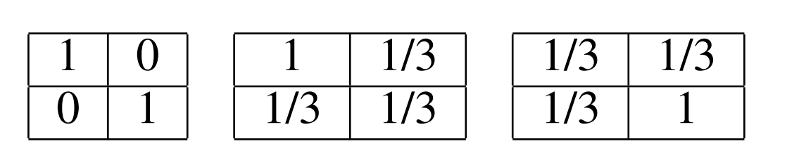
Table 1. Non-monotonic reward matrix (left) and two possible solutions returned by the QMIX operator (middle and right)

This phenomenon arises because the operator solves the problem within the \(\mathcal{Q}^{mix}\) space, whose key characteristic is “monotonicity”. When the fixed point exhibits “non-monotonicity”, it lies outside \(\mathcal{Q}^{mix}\), forcing the algorithm to find approximate solutions (such as the two solutions in Table 1).

Since contraction mappings are defined on complete metric spaces, the QMIX operator \(`\mathcal{T}_{\mathrm{Qmix}}^*`\) — defined on the \(`\mathcal{Q}^{mix}`\) space — is not a contraction mapping.

This provides a deeper explanation of QMIX’s limitations.

Property 2: The joint action maximized by \(Q_{tot}\) in QMIX is not always correct.

The authors note that there may exist Q-functions for which \(\arg\max\Pi_{\mathrm{Qmix}}Q\neq\arg\max Q\). If you understand Property 1, this property will be intuitive.

For example, consider a 2-agent, 3-action task.The left matrix in Table 2 is the true reward matrix \(`Q^*`\), and the right matrix is a \(`Q_{tot}`\) returned by the \(`\Pi_{\mathrm{Qmix}}`\) operator. According to \(`Q^*`\), the agent pair can obtain the maximum reward \(r = 8\) by selecting the corresponding action combination. However, to satisfy the “monotonicity constraint”, \(\Pi_{\mathrm{Qmix}}Q^*\) may fit the reward at the \(r = 8\) position to \(-12\), leaving the agents with a maximum achievable reward of \(r = 0\).

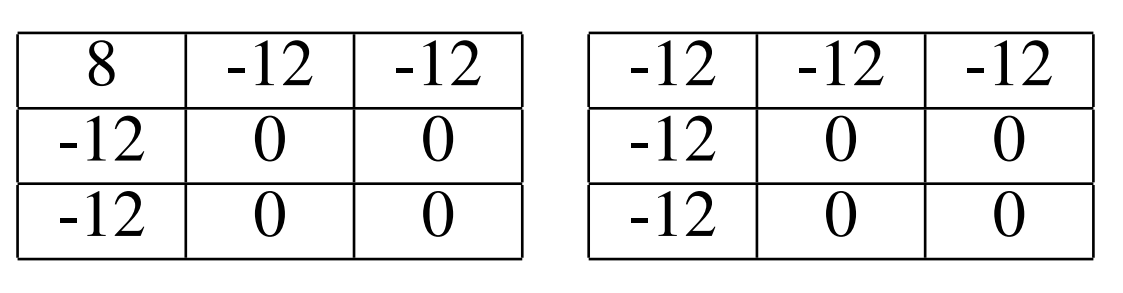
Table 2. True reward matrix (left) and the reward matrix returned by the QMIX operator (right).

This phenomenon also stems from the limitations of the \(\mathcal{Q}^{mix}\) function space.

Property 3: QMIX may underestimate the value of certain joint actions.

This property is closely related to Property 2. Incorrect argmax calculations inevitably lead to further errors in value function estimation. For example, the reward of \(r = 8\) in Table 2 is incorrectly estimated as \(-12\).

These three properties are inherent flaws of the QMIX algorithm and are unrelated to computational performance, exploration mechanisms, or network parameter settings.

Even under ideal conditions, QMIX exhibits such significant flaws. In practical training — where more uncontrollable factors exist — the situation may be even worse.

The Weighted QMIX Operator

Now that we have identified QIMX’s flaws, we can address them directly. The authors’ reasoning is as follows:

The optimization problem in Equation\(`(1)`\) iterates over all states in the state space and all actions in the joint action space. The authors argue that if the true reward is “non-monotonic”, it is unreasonable to sum all action values with equal weights (i.e., uniform weighting).

Take the right matrix in Table 2 as an example. Since \(Q_{tot}\) must satisfy the monotonicity constraint, the algorithm can only adjust action values in two ways to correct the incorrect estimation of \(-12\) to \(8\) : either increase the action values corresponding to \(r = -12\) (suboptimal actions) or decrease the action values corresponding to \(r = 0\) (second-best actions). Both options increase the overall error, so \(Q_{tot}\) avoids such adjustments and settles for a suboptimal solution.

Based on this insight, the authors propose weighting individual action values to mitigate the impact of such adjustments on overall error.

By adding a weight function \(w\) to the \(\Pi_{\mathrm{Qmix}}\) operator, a new operator is derived:

\[ \Pi_wQ:=\arg\min_{q\in\mathcal{Q}^{mix}}\sum_{\boldsymbol{u}\in U}w(s,\boldsymbol{u})(Q(s,\boldsymbol{u})-q(s,\boldsymbol{u}))^2.(5) \]

Here, the weight function \(w\) : \(S\times U\to(0,1]\) weights the importance of each joint action in QMIX’s loss function. The input space of \(w\) is not limited to state-joint action pairs; other factors can also be incorporated. Notably, when \(w(s,\boldsymbol{u})\equiv1\), \(\Pi_{w}\Leftrightarrow\Pi_{\mathrm{Qmix}}\).

Selection of the Weight Function \(w(s,\boldsymbol{u})\)

First Weight Function: Idealised Central Weighting

This weighting method is straightforward but requires iterating over the entire joint action space to compute \(\arg\max\), making it impractical for real-world use. As discussed later, the authors use approximation methods to address this issue during actual training.

The paper provides the following conclusion for this weight function:

Theorem 1. Let \(w\) be the Idealised Central Weighting defined in Equation\(`(6)`\). \(\exists\alpha>0\) such that \(\arg\max\Pi_wQ=\arg\max Q\) for any \(Q\).

This theorem guarantees the existence of “Idealised Central Weighting”, ensuring that \(\arg\max\Pi_wQ\) does not produce incorrect actions (unlike QMIX).

Second Weight Function: Optimistic Weighting

This weight function assigns a higher weight (\(1\)) to all underestimated action values and a lower weight (\(\alpha\)) to all overestimated action values. This ensures that action values are estimated as accurately as possible, hence the name “Optimistic Weighting”.

Similarly, the authors provide the following conclusion for this weight function:

Theorem 2. Let \(w\) be the Idealised Central Weighting defined in Equation\(`(7)`\). \(\exists\alpha>0\) such that \(\arg\max\Pi_wQ=\arg\max Q\) for any \(Q\).

Theorem 2 also guarantees the existence of “Optimistic Weighting”, ensuring that the argmax operation on \(Q_{tot}\) does not produce incorrect actions.

Due to space constraints, the proofs of Theorem 1 and Theorem 2 are not detailed here; please refer to the supplementary materials in the original paper.

The Weighted QMIX Operator

According to the conclusions of Theorem 1 and Theorem 2, the two weight functions above ensure the accuracy of joint action output for any Q-function (including \(Q^*\)).

The design of both weight functions requires \(Q^*\) for computation. Thus, an additional \(`\hat{Q}^{*}`\) (to approximate \(`Q^*`\)) must be learned. However, computing \(`\arg\max\hat{Q}^{*}`\) during fitting requires searching the entire joint action space — a computationally infeasible task. To address this, the authors leverage the “monotonicity” of \(`Q_{tot}`\) nd propose using \(`\arg\max Q_{tot}`\) to generate actions, which are then estimated by \(`\hat{Q}^{*}`\).

The \(\hat{Q}^{*}\) function is updated using the following operator:

Comparing Equation \(`(8)`\) with Equation \(`(2)`\) (introduced earlier), the key difference between \(`\mathcal{T}_w^*`\) and \(`\mathcal{T}^*`\) is

that \(`\mathcal{T}_w^*`\) does not select actions by directly maximizing \(`\hat{Q}^{*}`\) ;

instead, it maximizes the monotonic function \(`Q_{tot}\in\mathcal{Q}^{mix}`\). Note that when \(`w(s,\boldsymbol{u})\equiv1`\), \(`\Pi_w\nLeftrightarrow\Pi_{\mathrm{Qmix}}`\).

Similarly, \(Q_{tot}\) is updated using the following operator:

This \(\mathcal{T}_{\mathrm{WQMIX}}^*\) is the Weighted QMIX operator.

To ensure that \(\mathcal{T}_{\mathrm{WQMIX}}^*\) converges to the optimal policy, the authors provide the following conclusion:

Corollary 1. Letting \(`w`\) be the Idealised Central or Optimistic Weighting, then \(`\exists\alpha>0`\) such that the unique fixed point of \(`\mathcal{T}_w^*`\) is \(`Q_{tot}`\). Furthermore, \(`\Pi_{w}Q^{*}\subseteq\mathcal{Q}^{mix}`\) recovers an optimal policy, and \(`\max\Pi_wQ^*(s,\cdot)=\max Q^*(s,\cdot)`\).

Algorithm Design

The above analysis of WQMIX assumes ideal conditions. Below, we discuss how to implement WQMIX using deep neural networks under partial observability.

Based on the preceding analysis, the WQMIX algorithm consists of three components: \(Q_{tot}\), \(\hat{Q}^*\) and \(w(s,\boldsymbol{u})\). The algorithm framework is shown in Figure 1.

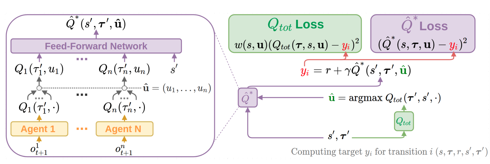
Figure 1. Implementation of the Weighted QMIX algorithm in the deep reinforcement learning setting.

The \(Q_{tot}\) Function

The structural design of \(Q_{tot}\) is nearly identical to that in the original QMIX algorithm. It is trained by minimizing the following loss:

Here, \(y_{i}:=r+\gamma\hat{Q}^{*}(s^{\prime},\boldsymbol{\tau}^{\prime},\arg\max_{\boldsymbol{u}^{\prime}}Q_{tot}(\boldsymbol{\tau}^{\prime},\boldsymbol{u}^{\prime},s^{\prime}))\)

The \(\hat{Q}^*\) Function

The authors implement \(`\hat{Q}^*`\) using a structure similar to QMIX (see the left panel of Figure 1). However, the Mixing Network in QMIX is replaced with a standard Feed-Forward Network. This network takes the Q-functions of all agents \(`\{Q_i(\tau_i^{\prime},u_i)\}_{i=1}^n`\) and the global state \(`s^{\prime}`\) as inputs, and outputs \(`\hat{Q}^*`\).

The \(\hat{Q}^*\) function is trained by minimizing the following loss function:

The computation of \(y_i\) is identical to that in Equation\(`(10)`\).

The Weight Function \(w(s,\boldsymbol{u})\)

Computing both weight functions requires maximizing \(\hat{Q}^*\) over the joint action space, which is computationally expensive when the number of agents is large. Thus, the authors use approximation methods to solve this problem.

Centrally-Weighted QMIX (CW-QMIX)

Here, \(`\boldsymbol{\hat{u}}^{*}=\arg\max_{\boldsymbol{u}}Q_{tot}(\boldsymbol{\tau},\boldsymbol{u},s)`\). If \(`y_{i}>\hat{Q}^{*}(s,\boldsymbol{\tau}`\), \(`u`\) can be approximately regarded as the optimal joint action.

Compared with Equation\(`(6)`\), Equation\(`(12)`\) replaces \(`\mathcal{T}_w^*\hat{Q}^{*}(s,\boldsymbol{\tau},\boldsymbol{\hat{u}^{*}})`\) with \(`\hat{Q}^{*}(s,\boldsymbol{\tau},\boldsymbol{\hat{u}^{*}})`\). The Weighted QMIX algorithm based on Equation\(`(12)`\) is called “Centrally-Weighted QMIX (CW-QMIX)”.

Optimistically-Weighted QMIX (OW-QMIX)

The Weighted QMIX algorithm based on Equation\(`(13)`\) is called “Optimistically-Weighted QMIX (OW-QMIX)”. Unlike Equation\(`(7)`\), it requires no approximation.

The above covers the theoretical and design aspects of the Weighted QMIX algorithm. Instead of modifying QMIX’s “monotonicity constraint” to enhance its function representation capability, WQMIX uses a weight function to weight each action in the joint action space based on its importance. This allows monotonic functions (satisfying QMIX’s constraints) to be mapped to non-monotonic functions via the Weighted QMIX operator.

Conclusion

This paper addresses the limitations of QMIX’s function representation capability. Through an analysis of QMIX under ideal conditions, the authors propose the Weighted QMIX algorithm. Theoretically, WQMIX guarantees that monotonic functions (output by QMIX) can be mapped to non-monotonic value functions via action weighting. This enables WQMIX to learn the optimal policy and avoids QMIX’s tendency to converge to suboptimal policies.

To learn the weight function, WQMIX also learns a \(`\hat{Q}^*`\) function that is not constrained by “monotonicity”, ensuring its convergence to \(`Q^*`\). However, in practical training, approximation methods and the design of the \(`\hat{Q}^*`\) structure may lead to performance degradation.

The authors note that WQMIX has room for further improvement — particularly in the design of weight functions. The weight functions used in this paper are simple, considering only global state and joint action information, and taking values of either 1 or \(\alpha\). Thus, more complex weight functions represent a promising future research direction for WQMIX.

Run WQMIX in XuanCe

Before running WQMIX in XuanCe, you need to prepare a conda environment and install xuancefollowing the installation steps.

Run Build-in Demos

After completing the installation, you can open a Python console and run WQMIX directly using the following commands:

import xuance
runner = xuance.get_runner(algo='wqmix',
                           env='mpe',  # Choices: football, mpe, sc2
                           env_id='simple_spread_v3',  # Choices: simple_spread_v3, etc
                           )
runner.run()

Run With Self-defined Configs

If you want to run WQMIX with different configurations, you can build a new .yaml file, e.g., my_config.yaml. Then, run the WQMIX by the following code block:

import xuance as xp
runner = xp.get_runner(algo='wqmix',
                       env='mpe',  # Choices: football, mpe, sc2
                       env_id='simple_spread_v3',  # Choices: simple_spread_v3, etc
                       config_path="my_config.yaml",  # The path of my_config.yaml file should be correct.
                       )
runner.run()  # Or runner.benchmark()

To learn more about the configurations, please visit the tutorial of configs.

Run With Custom Environment

If you would like to run XuanCe’s QMIX in your own environment that was not included in XuanCe, you need to define the new environment following the steps in New Environment Tutorial. Then, prepapre the configuration file wqmix_myenv.yaml.

After that, you can run WQMIX in your own environment with the following code:

import argparse
from xuance.common import load_yaml
from xuance.environment import REGISTRY_ENV
from xuance.environment import make_envs
from xuance.torch.agents import WQMIX_Agents

configs_dict = load_yaml(file_dir="wqmix_myenv.yaml")
configs = argparse.Namespace(**configs_dict)
REGISTRY_ENV[configs.env_name] = MyNewEnv

envs = make_envs(configs)  # Make parallel environments.
Agent = WQMIX_Agents(config=configs, envs=envs)  # Create WQMIX agents from XuanCe.
Agent.train(configs.running_steps // configs.parallels)  # Train the model for numerous steps.
Agent.save_model("final_train_model.pth")  # Save the model to model_dir.
Agent.finish()  # Finish the training.

Citation

@article{rashid2020weighted,
  title={Weighted qmix: Expanding monotonic value function factorisation for deep multi-agent reinforcement learning},
  author={Rashid, Tabish and Farquhar, Gregory and Peng, Bei and Whiteson, Shimon},
  journal={Advances in neural information processing systems},
  volume={33},
  pages={10199--10210},
  year={2020}
}