SPR: Self-Predictive Representations for Reinforcement Learning¶

Paper Link: ArXiv

Self-Predictive Representations (SPR) is an off-policy deep reinforcement learning algorithm that learns representations by predicting future states in latent space. SPR combines the benefits of contrastive methods like CURL with predictive methods, enabling more efficient learning from high-dimensional visual inputs. It addresses the issue of sample inefficiency that commonly occurs when applying reinforcement learning to pixel-based control tasks by learning rich state representations that capture temporal dependencies.

This table lists some general features about SPR algorithm:

Features of SPR	Values	Description
On-policy	❌	The evaluate policy is the same as the target policy.
Off-policy	✅	The evaluate policy is different from the target policy.
Model-free	✅	No need to prepare an environment dynamics model.
Model-based	❌	Need an environment model to train the policy.
Discrete Action	✅	Deal with discrete action space.
Continuous Action	❌	Deal with continuous action space.

Algorithm Description¶

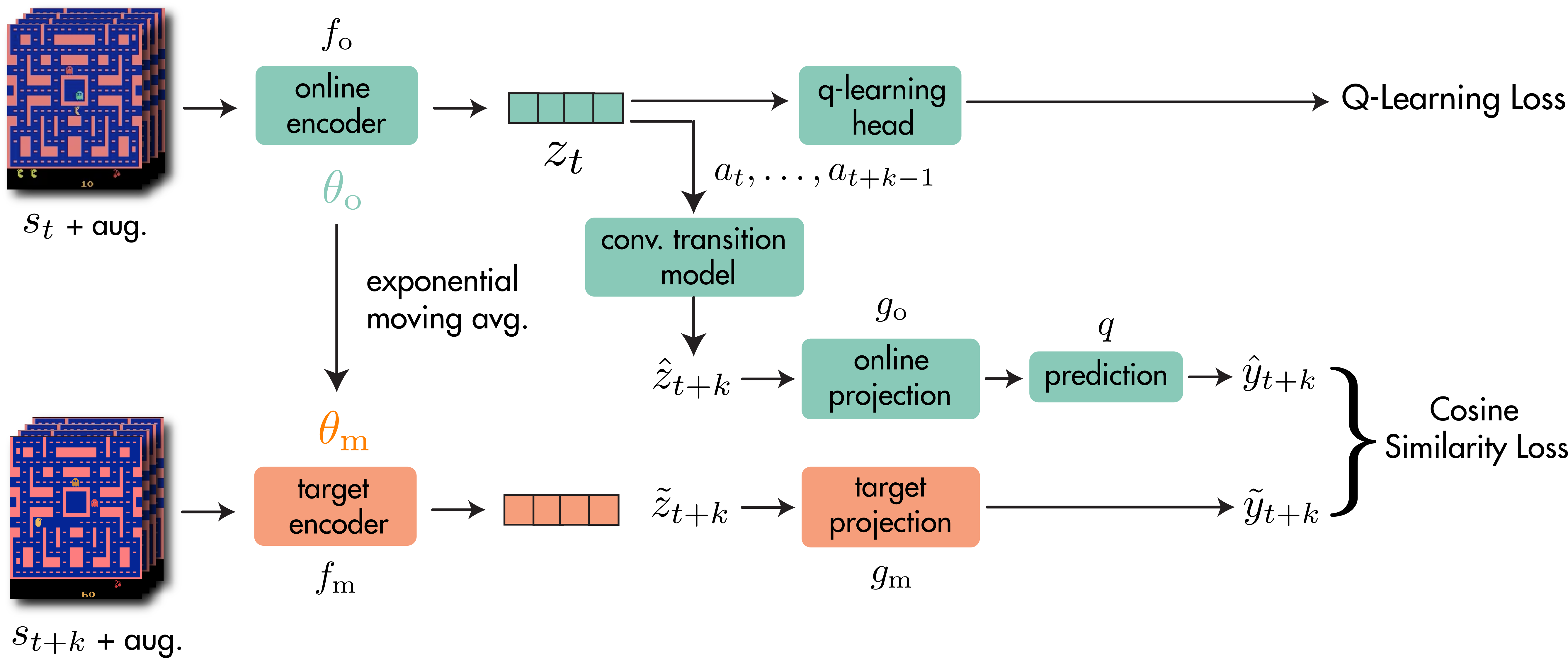
SPR addresses the challenge of sample inefficiency in reinforcement learning from pixels by learning temporally predictive representations. The main idea is to train a convolutional encoder to predict its own latent state representations multiple steps into the future. This approach encourages the encoder to learn representations that capture the essential features of the environment dynamics while being invariant to task-irrelevant details.

The key insight is that by predicting future states in latent space, SPR learns representations that are both predictive and stable. This enables more efficient learning of the policy since the agent can make better use of past experiences by understanding how the environment evolves over time.

Network Architecture¶

The SPR agent uses a convolutional neural network (CNN) as the backbone of the representation network. The architecture typically consists of several convolutional layers followed by fully connected layers. The encoder network maps observations to latent representations, which are then used by the Q-network to estimate Q-values.

SPR extends the encoder with a transition model that predicts future latent states. This transition model takes the current latent state and a sequence of actions as input, and outputs predictions of future latent states.

Implementation Details¶

Agent Implementation¶

class SPR_Agent(OffPolicyAgent):
    def __init__(self, 
                 config: Namespace,
                 envs: Union[DummyVecEnv, SubprocVecEnv]):
        super(SPR_Agent, self).__init__(config, envs)
        self._init_exploration_params(config)
        
        self.policy = self._build_policy()  # build policy
        self.memory = self._build_memory()  # build memory
        self.learner = self._build_learner(config, self.policy)  # build learner
        self.transform = SPR_Augmentations.get_transform(self.observation_space.shape[-1])

    def _init_exploration_params(self, config: Namespace):
        self.e_greedy = config.start_greedy
        self.e_greedy_decay = (config.start_greedy - config.end_greedy) / (config.decay_step_greedy / self.n_envs)

Encoder and Transition Model¶

The SPR encoder maps observations to latent representations. A transition model predicts future representations based on current representations and actions:

class SPR_Encoder(nn.Module):
    """SPR encoder (CNN architecture)"""
    
    def __init__(self, observation_space: Space, config: Namespace, device: str):
        super().__init__()
        self.device = device
        self.net = nn.Sequential(
            nn.Conv2d(4, 32, kernel_size=8, stride=4),
            nn.ReLU(),
            nn.Conv2d(32, 64, kernel_size=4, stride=2),
            nn.ReLU(),
            nn.Conv2d(64, 64, kernel_size=3, stride=1),
            nn.Flatten(),
            nn.Linear(64 * 7 * 7, 512),
            nn.LayerNorm(512)
        )

    def forward(self, x: torch.Tensor):
        x = x.permute(0, 3, 1, 2)  # (B, H, W, C) -> (B, C, H, W)
        return self.net(x)

Training Process¶

The training process of SPR involves the following steps:

Collect experiences from the environment
Apply data augmentations to observations
Update the representation network using both contrastive and predictive losses
Update the Q-network using the learned representations
Periodically update the target networks

The SPR loss combines a contrastive loss (similar to CURL) and a predictive loss:

\[ \mathcal{L}_{\text{SPR}} = \mathcal{L}_{\text{contrastive}} + \lambda \mathcal{L}_{\text{predictive}} \]

where \(\lambda\) is a weighting factor that balances the two losses.

The predictive loss encourages the transition model to accurately predict future representations:

\[ \mathcal{L}_{\text{predictive}} = \sum_{k=1}^{K} \| \hat{z}_{t+k} - z_{t+k} \|_2^2 \]

where \(\hat{z}_{t+k}\) is the predicted representation at time \(t+k\), \(z_{t+k}\) is the actual representation, and \(K\) is the number of prediction steps.

Key Features¶

Temporal Predictive Learning¶

SPR learns representations by predicting future states in latent space. This temporal predictive learning encourages the encoder to capture the essential dynamics of the environment, leading to more informative representations.

Data Efficiency¶

By learning rich representations that capture temporal dependencies, SPR significantly improves sample efficiency compared to standard Q-learning methods. The agent can make better use of past experiences by understanding how the environment evolves over time.

Robustness¶

The combination of contrastive and predictive learning makes the learned representations more robust to variations in the input observations. This robustness is particularly important in real-world applications where the visual input may vary due to lighting conditions, camera angles, or other factors.

Advantages¶

Improved Sample Efficiency: SPR significantly improves sample efficiency by learning predictive representations.
Temporal Understanding: The predictive component enables the agent to understand temporal dynamics.
Robust Representations: Combining contrastive and predictive learning leads to more robust representations.

Application Scenarios¶

SPR is particularly well-suited for:

Pixel-based control tasks where the agent must learn from high-dimensional visual inputs
Environments where sample efficiency is critical
Applications where understanding temporal dynamics is important

Algorithm¶

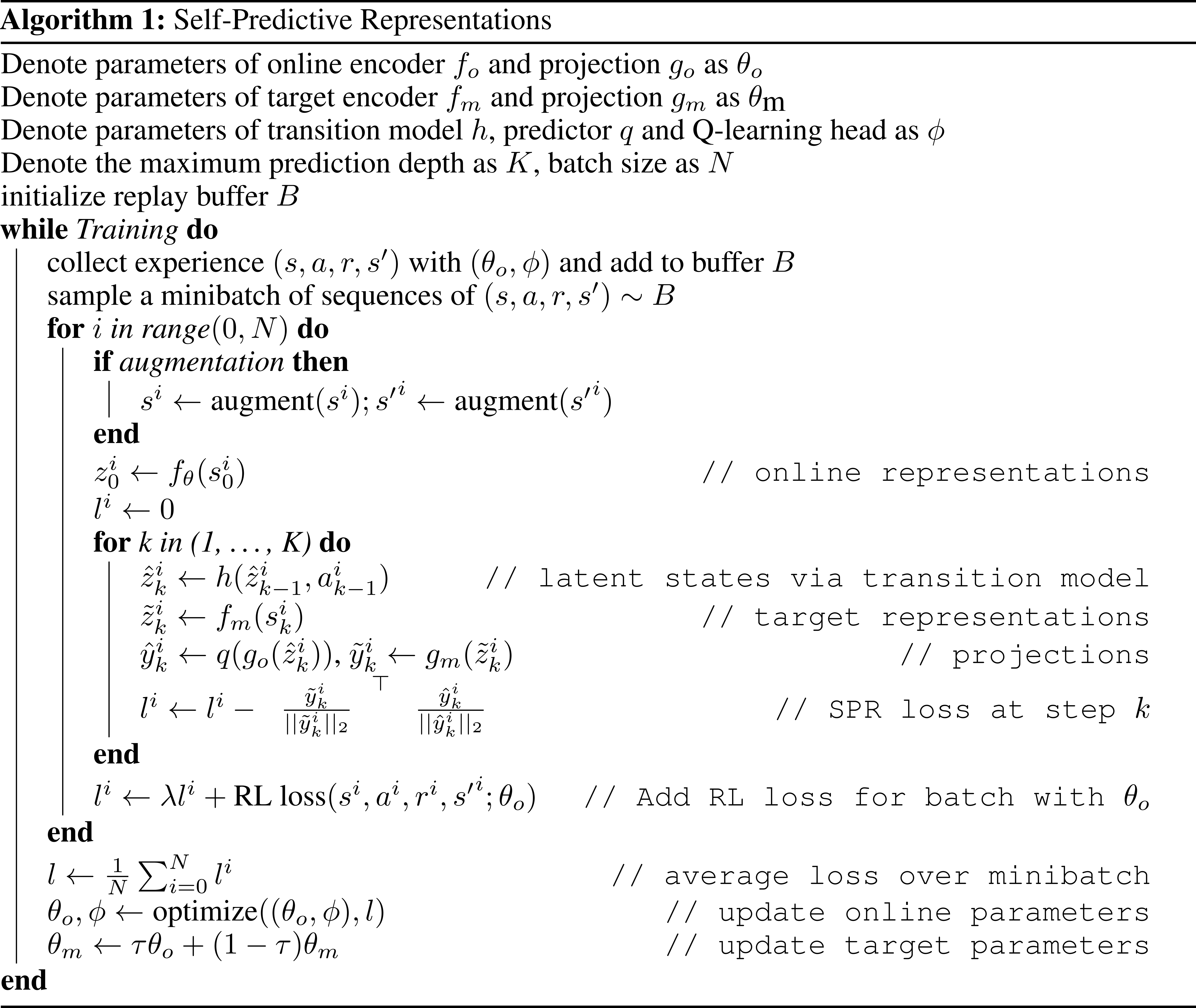
The full algorithm for training SPR is presented in Algorithm 1:

Framework¶

The overall agent-environment interaction of SPR, as implemented in XuanCe, is illustrated in the figure below.

Run SPR in XuanCe¶

Before running SPR in XuanCe, you need to prepare a conda environment and install xuance following the installation steps.

Run Build-in Demos¶

After completing the installation, you can open a Python console and run SPR directly using the following commands:

import xuance
runner = xuance.get_runner(algo='spr',
                           env='atari',  # Currently only atari environments are supported.
                           env_id='ALE/Breakout-v5',  # Choices: ALE/Breakout-v5, ALE/Pong-v5, etc.
                           )
runner.run()  # Or runner.benchmark()

Run With Self-defined Configs¶

If you want to run SPR with different configurations, you can build a new .yaml file, e.g., my_config.yaml. Then, run the SPR by the following code block:

import xuance
runner = xuance.get_runner(algo='spr',
                       env='atari',  # Currently only atari environments are supported.
                       env_id='ALE/Breakout-v5',  # Choices: ALE/Breakout-v5, ALE/Pong-v5, etc.
                       config_path="my_config.yaml",  # The path of my_config.yaml file should be correct.
                       )
runner.run()  # Or runner.benchmark()

To learn more about the configurations, please visit the tutorial of configs.

Citations¶

@inproceedings{raileanu2021spr,
  title={Self-predictive representation learning},
  author={Raileanu, Robert and Fergus, Rob},
  booktitle={International Conference on Learning Representations},
  year={2021}
}