Multi-agent Deep Deterministic Policy Gradient (MADDPG)¶

Paper Link: https://arxiv.org/abs/1706.02275

Multi-agent deep deterministic policy gradient (MA-DDPG) is a multi-agent deep reinforcement learning algorithm which consider DDPG algorithm as the baseline and centralized training and decentralized execution as the training method. This method is applicable not only to cooperative interaction, but also to competitive or mixed interaction involving both physical and communicative behavior.

This table lists some general features about MADDPG algorithm:

Features of MADDPG	Values	Description
Fully Decentralized	❌	There is no communication between agents.
Fully Centralized	❌	Agents send all information to the central controller, and the controller will make decisions for all agents.
Centralized Training With Decentralized Execution(CTDE)	✅	The central controller is used in training and abandoned in execution.
On-policy	❌	The evaluate policy is the same as the target policy.
Off-policy	✅	The evaluate policy is different from the target policy.
Model-free	✅	No need to prepare an environment dynamics model.
Model-based	❌	Need an environment model to train the policy.
Discrete Action	✅	Deal with discrete action space.
Continuous Action	✅	Deal with continuous action space.

Framework¶

The following figure shows the algorithm structure of MADDPG.

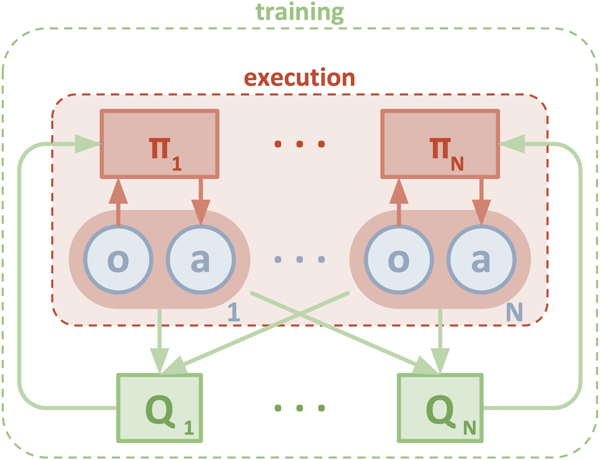
Where \(\pi=(\pi_1,\ldots,\pi_N)\) represents the strategy of N agents,which are respectively fitted by N Actor networks with parameter \(\theta=(\theta_1,\ldots,\theta_N).\)

Key Ideas of MADDPG¶

Multi-Agent Actor Critic¶

MADDPG operate under the following constraints:

The learned policies can only use local information(their own observation) at execution time.
It does not assume a differentiable model of the environment dynamics.
It does not assume any particular structure on the communication method between agents(it doesn’t assume a differentiable communication channel).

Based on the above constraints,we can write the gradient of the expected return for agent \(i\), \(J \left( \theta_i \right)=\mathbb{E} \left( R_i \right)\) as:

\[ \nabla_{\theta_i} J \left( \theta_i \right) = \mathbb{E}_{s \sim p^\mu,a_i \sim \pi_i} \left[ \nabla_{\theta_i} \log \pi_i \left( a_i \left| o_i \right. \right) Q_i^\pi\left(x,a_1,\ldots,a_N\right) \right] \]

Where \(Q_i^\pi\left(x,a_1,\ldots,a_N\right)\) is a centralized action-value function.Besides state information \(x\),it also takes all actions of agent \(a_1,\ldots,a_N\) as input, and finally outputs the Q-value of agent \(i\) . For \(x=(o_1,\ldots,o_N,\mathrm{X})\),it could consist of the observations of all agents, and other useful additional information that may exist.
For deterministic policy gradient,we could consider N continuous policies \(\mu_{\theta_i}\) ,then the gradient can be written as:

\[ \nabla_{\theta_{i}}J\left(\mu_{\theta_{i}}\right)=\mathbb{E}_{x,a\sim D}\left[\nabla_{\theta_{i}}\mu_{\theta_{i}}\left(a_{i}\left|o_{i}\right)\nabla_{a_{i}}Q_{i}^{\mu}\left(x,a_{1},\ldots,a_{N}\left|\right._{a_{i}=\mu_{\theta_{i}}(o_{i})}\right)\right]\right. \]

Where the experience replay buffer \(D\) contains the data \((x,x^{\prime},a_1,\ldots,a_N,r_1,\ldots,r_N)\) ,which includes the experience of all agents.
For the centralized action-value function \(Q_i^\mu\) ,it can be updated with the following loss function:

\[ L\left(\theta_i\right)=\mathbb{E}_{x,a,r,x^{\prime}}\left[\left(Q_i^\mu\left(x,a_1,\ldots,a_N\right)-y\right)^2\right] \]

Where \(y=r_i+\gamma{Q_i}^{\mu^\prime}(x^\prime,a_1^\prime,\ldots,a_N^\prime)\left|\right._{a^\prime_j=\mu^\prime_j(o_j)}\), in the y equation, \(\mu^\prime=(\mu_{\theta_1}^\prime,\ldots,\mu_{\theta_N}^\prime)\) is the set of target policies used in updating the value function.

Agents with Policy Ensembles¶

An important problem of multi-agent reinforcement learning is that the environment is non-stationarity because of the constant changes of other agents’ policies,especially in a competitive setting.
In order to solve this problem,the author puts forward the concept of policy ensembles training,which trains \(K\) different sub-policies and then randomly selects one particular sub-policy for each agent to execute at each episode. For agent \(i\),its objective function can be changed to:

\[ J_e\left(\mu_i\right)=\mathbb{E}_{k\sim unif(1,K),s\sim p^\mu,a\sim\mu_i^{(k)}}\left[R_i\left(s,a\right)\right] \]

Where \(unif\left(1,K\right)\) represents the sub-policy index set, \(K\) represents the sub-policy index. Then the corresponding policy gradient can be rewritten as:

\[ \nabla_{\theta_{i}^{(k)}}J_{e}\left(\mu_{\theta_{i}}\right)=\frac{1}{K}\mathbb{E}_{x,a\sim D_{i}^{(k)}}\left[\nabla_{\theta_{i}^{(k)}}\mu_{\theta_{i}^{(k)}}\left(a_{i}\left|o_{i}\right)\nabla_{a_{i}}Q^{\mu_{i}}\left(x,a_{1},\ldots,a_{N}\right|_{a_{i}=\mu_{\theta_{i}^{(k)}}(o_{i})}\right)\right] \]

Algorithm¶

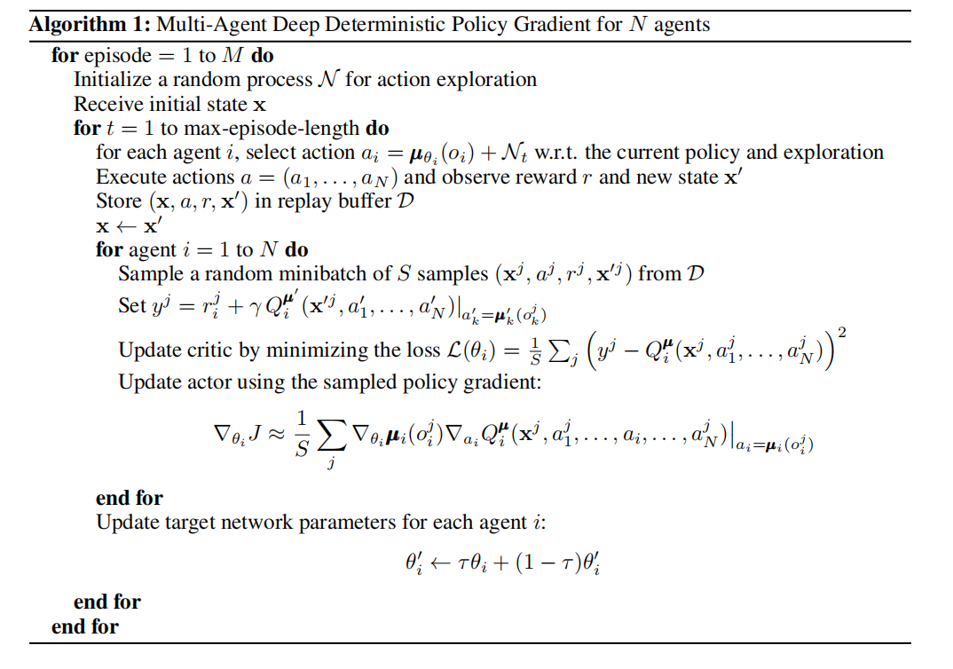
The full algorithm for training MADDPG is presented in Algorithm 1:

Run MADDPG in XuanCe¶

Before running MADDPG in XuanCe, you need to prepare a conda environment and install xuance following the installation steps.

Run Build-in Demos¶

After completing the installation, you can open a Python console and run MADDPG directly using the following commands:

import xuance
runner = xuance.get_runner(algo='maddpg',
                           env='mpe',  # Choices: mpe, Drones, NewEnv_MAS.
                           env_id='simple_spread_v3',  # Choices: simple_spread_v3, etc.
                           )
runner.run()  # Or runner.benchmark()

For competitve tasks in which agents can be divided to two or more sides, you can run a demo by:

import xuance
runner = xuance.get_runner(algo=["maddpg", "iddpg"],
                           env='mpe',  # Choices: mpe.
                           env_id='simple_push_v3',  # Choices: simple_adversary_v3, simple_push_v3, etc.
                           )
runner.run()

In this demo, the agents in mpe/simple_push_v3 environment are divided into two sides, named “adversary_0” and “agent_0”. The “adversary”s are MADDPG agents, and the “agent”s are IDDPG agents.

Run With Self-defined Configs¶

If you want to run MADDPG with different configurations, you can build a new .yaml file, e.g., my_config.yaml. Then, run the MADDPG by the following code block:

import xuance
runner = xuance.get_runner(algo='maddpg',
                       env='mpe',  # Choices: mpe, Drones, NewEnv_MAS.
                       env_id='simple_spread_v3',  # Choices: simple_spread_v3, etc.
                       config_path="my_config.yaml",  # The path of my_config.yaml file should be correct.
                       )
runner.run()  # Or runner.benchmark()

To learn more about the configurations, please visit the tutorial of configs.

Run With Custom Environment¶

If you would like to run XuanCe’s MADDPG in your own environment that was not included in XuanCe, you need to define the new environment following the steps in New Environment Tutorial. Then, prepapre the configuration file maddpg_myenv.yaml.

After that, you can run MADDPG in your own environment with the following code:

import argparse
from xuance.common import load_yaml
from xuance.environment import REGISTRY_ENV
from xuance.environment import make_envs
from xuance.torch.agents import MADDPG_Agents

configs_dict = load_yaml(file_dir="maddpg_myenv.yaml")
configs = argparse.Namespace(**configs_dict)
REGISTRY_ENV[configs.env_name] = MyNewEnv

envs = make_envs(configs)  # Make parallel environments.
Agent = MADDPG_Agents(config=configs, envs=envs)  # Create a MADDPG agent from XuanCe.
Agent.train(configs.running_steps // configs.parallels)  # Train the model for numerous steps.
Agent.save_model("final_train_model.pth")  # Save the model to model_dir.
Agent.finish()  # Finish the training.

Citation¶

@article{lowe2017multi,
  title={Multi-Agent Actor-Critic for Mixed Cooperative-Competitive Environments},
  author={Lowe, Ryan and Wu, Yi and Tamar, Aviv and Harb, Jean and Abbeel, Pieter and Mordatch, Igor},
  journal={Neural Information Processing Systems (NIPS)},
  year={2017}
}