Counterfactual Multi-agent Policy Gradient (COMA)¶

Paper Link: https://ojs.aaai.org/index.php/AAAI/article/view/11794.

Counterfactual Multi - Agent Policy Gradient (COMA) is a reinforcement learning algorithm for multi - agent collaboration problems. It aims to improve the learning performance of decentralized agents by reducing the variance of policy gradients.

It was first proposed by the DeepMind team. The title of the paper is “Counterfactual Multi - Agent Policy Gradients”, which was published by Jakob Foerster and others at the AAAI conference in 2017. It is applicable to multi - agent environments with local observations and decentralized decision - making, especially for cooperation problems under policy gradient methods.

This table lists some general features about COMA algorithm:

Features of COMA	Values	Description
Fully Decentralized	❌	There is no communication between agents.
Fully Centralized	❌	Agents send all information to the central controller, and the controller will make decisions for all agents.
Centralized Training with Decentralized Execution (CTDE)	✅	The central controller is used in training and abandoned in execution.
On-policy	✅	The evaluate policy is the same as the target policy.
Off-policy	❌	The evaluate policy is different from the target policy.
Model-free	✅	No need to prepare an environment dynamics model.
Model-based	❌	Need an environment model to train the policy.
Discrete Action	✅	Deal with discrete action space.
Continuous Action	❌	Deal with continuous action space.

Motivation¶

Partially observable and decentralized decision-making¶

In collaborative multi - agent systems, RL methods designed for single agents usually perform poorly in complex reinforcement learning tasks because the joint action space of agents grows exponentially with the number of agents. It is often necessary to re-sort to decentralised policies, in which each agent selects its own action conditioned only on its local action-observation history. Furthermore, partial observability and communica-tion constraints during execution may necessitate the use of decentralised policies even when the joint action space is not prohibitively large.

Credit Assignment¶

In cooperative set-tings, joint actions typically generate only global rewards,making it difﬁcult for each agent to deduce its own con-tribution to the team’s success. Sometimes it is possible to design individual reward functions for each agent. However,these rewards are not generally available in cooperative set-tings and often fail to encourage individual agents to sacri-ﬁce for the greater good. This often substantially impedes multi-agent learning in challenging tasks, even with rela-tively small numbers of agents.

Key Ideas¶

COMA considers a fully cooperative multi-agent task that can be described as a stochastic game $G$, defined by a tuple $G = \langle S, U, P, r, Z, O, n, \gamma \rangle$, in which $n$ agents identified by $a \in A \equiv \{1, \dots, n\}$ choose sequential actions. The environment has a true state $s \in S$. At each time step, each agent simultaneously chooses an action $u^a \in U$, forming a joint action $\mathbf{u} \in \mathbf{U} \equiv U^n$ which induces a transition in the environment according to the state transition function $P(s'|s, \mathbf{u}) : S \times \mathbf{U} \times S \to [0, 1]$. The agents all share the same reward function $r(s, \mathbf{u}) : S \times \mathbf{U} \to \mathbb{R}$ and $\gamma \in [0, 1)$ is a discount factor.

COMA considers a partially observable setting, in which agents draw observations $z \in Z$ according to the observation function $O(s, a) : S \times A \to Z$. Each agent has an action-observation history $\tau^a \in T \equiv (Z \times U)^*$, on which it conditions a stochastic policy $\pi^a(u^a|\tau^a) : T \times U \to [0, 1]$. It denotes joint quantities over agents in bold, and joints quantities over agents other than a given agent $a$ with the superscript $-a$.

The discounted return is $R_t = \sum_{l=0}^\infty \gamma^l r_{t+l}$. The agents’ joint policy induces a value function, i.e., an expectation over $R_t$, $V^\pi(s_t) = \mathbb{E}_{s_{t+1:\infty}, \mathbf{u}_{t:\infty}} [R_t | s_t]$, and an action-value function $Q^\pi(s_t, \mathbf{u}_t) = \mathbb{E}_{s_{t+1:\infty}, \mathbf{u}_{t+1:\infty}} [R_t | s_t, \mathbf{u}_t]$. The advantage function is given by $A^\pi(s_t, \mathbf{u}_t) = Q^\pi(s_t, \mathbf{u}_t) - V^\pi(s_t)$.

The key ideas of COMA are as follows:

The Centralized Training, Distributed Execution¶

This is a mainstream paradigm in modern multi - agent reinforcement learning. Training phase (Learning): Agents are allowed to access global information (such as maps and the positions of all units), and even share experiences among all agents. Execution phase (Execution): Each agent can only make decisions based on what it can observe locally.

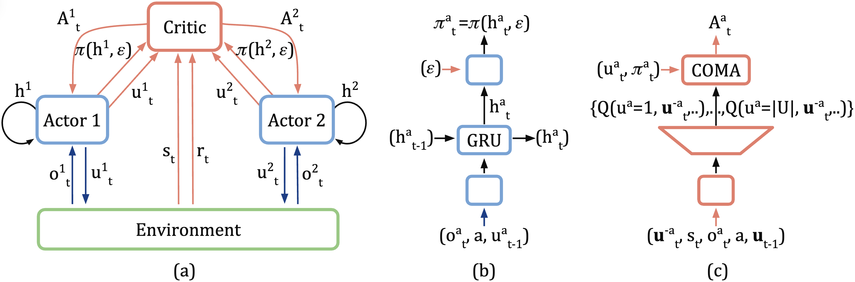
COMA takes advantage of this: Each agent has its own “actor” responsible for taking actions (decentralized execution).However, there is a unified “critic” with an omniscient perspective to evaluate the performance of the entire team.

A naive way to use this centralized critic is to let each actor update the gradient according to the TD - error estimated by this critic:

\[ g = \nabla_{\theta_{\pi}} \log \pi \left( u \mid \tau_{t}^{a} \right) \left( r + \gamma V(s_{t+1}) - V(s_{t}) \right) \]

Counterfactual Baseline¶

In the field of single - agent reinforcement learning, the advantage function is often used to measure the degree of advantage of a specific action compared to the average level. Its mathematical expression is: $$ A(s, a) = Q(s, a) - V(s) $$ where $Q(s, a)$ represents the return of taking action $a$ in state $s$, and $V(s)$ represents the average return of randomly taking actions in state $s$. That is, the advantage function is the difference between the return of taking a certain action and the average return of randomly taking actions.

However, in a multi - agent environment, due to the dynamic behaviors of other agents causing drastic environmental changes and high noise, the definition of the “average level” becomes ambiguous. To address this challenge, the COMA algorithm introduces the concept of a counterfactual baseline. This concept no longer focuses on the average level in the conventional sense but emphasizes the situation under counterfactual conditions: that is, whether the result will deteriorate if one agent changes its own action while the actions of other agents remain unchanged.

A key insight underlying COMA is that a centralised critic can be used to implement difference rewards in a way that avoids these problems. COMA learns a centralised critic, $Q(s, u)$ that estimates Q-values for the joint action $\mathbf{u}$ con-ditioned on the central state $s$. For each agent $a$ we can then compute an advantage function that compares the Q-value for the current action $u_a$ to a counterfactual baseline that marginalises out $\mathbf{u}_a$, while keeping the other agents’ actions $\mathbf{u}^{-a}$ ﬁxed: $$ A^a(s, \mathbf{u}) = Q(s, \mathbf{u}) - \sum_{u'^a} \pi^a(u'^a \mid \tau^a) \cdot Q\left(s, \left(\mathbf{u}^{-a}, u'^a\right)\right) $$

$A^a(s, \mathbf{u}^a)$ computes a separate baseline for eachagent that uses the centralised critic to reason about counter-factuals in which only a’s action changes, learned directly from agents’ experiences instead of relying on extra simula-tions, a reward model, or a user-designed default action. So, each agent can receive a fairer and more accurate feedback.

Framework¶

The following figure shows the algorithm structure of COMA.

Algorithm¶

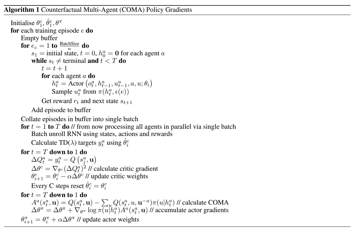
The full algorithm for training COMA is presented in Algorithm 1:

Run COMA in XuanCe¶

Before running COMA in XuanCe, you need to prepare a conda environment and install xuance following the installation steps.

Run Build-in Demos¶

After completing the installation, you can open a Python console and run COMA directly using the following commands:

import xuance
runner = xuance.get_runner(algo='coma',
                    env='mpe',  
                    env_id='simple_spread_v3',  
                    )
runner.run() 

Run With Self-defined Configs¶

If you want to run COMA with different configurations, you can build a new .yaml file, e.g., my_config.yaml. Then, run the COMA by the following code block:

import xuance
runner = xuance.get_runner(algo='coma',
                       env='mpe', 
                       env_id='simple_spread_v3',  
                       config_path="my_config.yaml",  # The path of my_config.yaml file should be correct.
                       )
runner.run()

Run With Custom Environment¶

If you would like to run XuanCe’s COMA in your own environment that was not included in XuanCe, you need to define the new environment following the steps in New Environment Tutorial. Then, prepapre the configuration file coma_myenv.yaml.

After that, you can run COMA in your own environment with the following code:

import argparse
from xuance.common import load_yaml
from xuance.environment import REGISTRY_ENV
from xuance.environment import make_envs
from xuance.torch.agents import COMA_Agents

configs_dict = load_yaml(file_dir="coma_myenv.yaml")
configs = argparse.Namespace(**configs_dict)
REGISTRY_ENV[configs.env_name] = MyNewEnv

envs = make_envs(configs)
Agent = COMA_Agents(config=configs, envs=envs)
Agent.train(configs.running_steps // configs.parallels)
Agent.save_model("final_train_model.pth")
Agent.finish()  # Finish the training.

Citation¶

@inproceedings{foerster2018counterfactual,
  title={Counterfactual multi-agent policy gradients},
  author={Foerster, Jakob and Farquhar, Gregory and Afouras, Triantafyllos and Nardelli, Nantas and Whiteson, Shimon},
  booktitle={Proceedings of the AAAI conference on artificial intelligence},
  volume={32},
  number={1},
  year={2018}
}