Value Decomposition Networks (VDN)¶

Paper Links:

Today, we introduce the VDN (Value Decomposition Networks) algorithm. I originally planned to present this algorithm together with QMIX, but given VDN’s reputation and influence in the field of MARL, I decided to introduce this one separately first. Additionally, as the predecessor of QMIX, an in-depth analysis of the VDN algorithm should help us understand the QMIX algorithm more thoroughly. In this way, we can also gain a more comprehensive understanding of the advantages and disadvantages of these two algorithms.

This table lists some general features about VDN algorithm:

Features of VDN	Values	Description
Fully Decentralized	❌	There is no communication between agents.
Fully Centralized	❌	Agents send all information to the central controller, and the controller will make decisions for all agents.
Centralized Training with Decentralized Execution (CTDE)	✅	The central controller is used in training and abandoned in execution.
On-policy	❌	The evaluate policy is the same as the target policy.
Off-policy	✅	The evaluate policy is different from the target policy.
Model-free	✅	No need to prepare an environment dynamics model.
Model-based	❌	Need an environment model to train the policy.
Discrete Action	✅	Deal with discrete action space.
Continuous Action	❌	Deal with continuous action space.

I. Problem Background and Research Approach¶

Similar to COMA, this work addresses the multi-agent reinforcement learning problem in cooperative tasks, meaning all agents share the same reward value (also referred to as the team reward). The difference is that VDN is a value function-based method, whereas COMA is based on policy gradients. In the previous introduction to COMA, we mentioned that agents sharing a team reward leads to the “credit assignment” problem—that is, the value function fitted using this team reward cannot evaluate the contribution of each agent’s policy to the overall outcome. This problem also exists in this paper.

The authors argue that since each agent has only local observations, the team reward received by one agent is likely caused by the actions of its teammates. In other words, this reward acts as a “spurious reward signal” for that agent. Therefore, each agent learning independently using reinforcement learning algorithms (i.e., independent RL) often yields poor performance.

Spurious rewards are also accompanied by a phenomenon termed “lazy agents” by the authors. When some agents in the team learn effective policies and can accomplish the task, other agents can obtain favorable team rewards without taking significant actions—these agents are referred to as “lazy agents.”

In essence, both “spurious rewards” and “lazy agents” stem from the credit assignment problem. If each agent optimizes its own objective function based on its actual contribution to the team, the aforementioned issues can be resolved. Driven by this motivation, the authors propose a research approach centered on “value function decomposition,” which decomposes the team’s global value function into N sub-value functions. These sub-value functions then serve as the basis for each agent’s action selection.

II. Algorithm Design¶

With the above approach in mind, the next step is to figure out how to decompose the value function. Here, the authors adopt the simplest method: summation.

2.1 Q-Function Value Decomposition¶

Assume that \(Q((h^1, h^2, \cdots, h^d), (a^1, a^2, \cdots, a^d))\) is the global Q-function of the multi-agent team, where \(d\) is the number of agents, \(h^i\) is the historical sequence information of agent \(i\), and \(a^i\) is its action. The input to this Q-function incorporates the observations and actions of all agents and can be iteratively fitted via the team reward \(r\). To derive the value function for each individual agent, the authors propose the following assumption:

\[ Q((h^1, h^2, \cdots, h^d), (a^1, a^2, \cdots, a^d)) \approx \sum_{i=1}^d \widetilde{Q}_i(h^i, a^i) . \quad(1) \]

This assumption indicates that the team’s Q-function can be approximately decomposed into \(d\) sub-Q-functions through summation, each corresponding to \(d\) distinct agents, the input of each sub-Q-function consists of the local observation sequence and action of its corresponding agent, and these sub-Q-functions are not influenced by one another, as illustrated in the figure below.

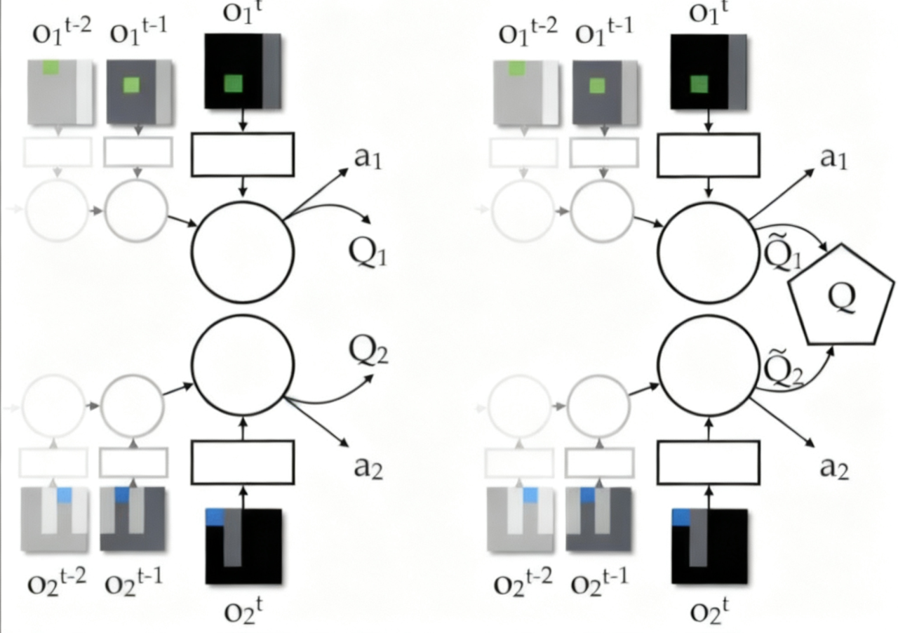
../../../_images/VDN_comparison.png — Figure 1. Left: independent RL; Right: VDN value decomposition.¶

Thus, each agent has its own value function and can make decisions based on its local value function:

\[ a^{i}=\arg\max_{a^{i\prime}}\tilde{Q}_{i}(h^{i},a^{i\prime}).\quad(2) \]

Note: Here, \(\tilde{Q}_i (h^i, a^i)\) is not a Q-value function in any strict sense, because there is no theoretical guarantee that there necessarily exists a reward function that makes this \(\tilde{Q}_i\) satisfy the Bellman equation.

2.2 Is This Decomposition Reasonable?¶

In fact, for Equation (1) to hold, at least one condition must be satisfied:

\[r(\mathbf{s}, \mathbf{a}) = \sum_{i=1}^d r(o^i, a^i) . \quad(3)\]

where \(\mathbf{s}\) represents the global state of the system, and \(\mathbf{a}\) denotes the joint action of all agents. Equation (3) indicates that the team’s global reward should be obtained by summing the individual reward functions of all agents. However, even if this condition is satisfied, according to the proof in the paper, the decomposition of the Q-function should be written as: \(Q(\mathbf{s}, \mathbf{a}) = \sum_{i=1}^d Q_i(\mathbf{s}, \mathbf{a})\). The input to each sub-Q-function should be the global state \(\mathbf{s}\) and the joint action \(\mathbf{a}\), rather than the form in Equation (1).

Therefore, this bug is a fundamental limitation of the VDN algorithm, to compensate for the constraints of local observations, the authors use the sequence of each agent’s historical observations, actions, and rewards as the input to its value function \(\tilde{Q}_i\).

Nevertheless, this setup ensures that each agent does not share the same value function, which to some extent alleviates the credit assignment problem.

Additionally, the structure of VDN enables end-to-end training. During centralized training, VDN only needs to compute the TD-error of the global Q-function and then backpropagate the error to each individual Q-function, significantly reducing computational complexity.

Summary¶

The VDN algorithm features a simple structure, the \(Q_i\) obtained through its decomposition allows agents to select greedy actions based on their local observations, thereby executing distributed policies. Its centralized training approach ensures the optimality of the global Q-function to some extent. Additionally, VDN’s “end-to-end training” and “parameter sharing” enable very fast algorithm convergence, for some simple tasks, this algorithm can be considered both fast and effective.

However, for larger-scale multi-agent optimization problems, its learning capability is significantly reduced. The fundamental limitation lies in the lack of theoretical support for the effectiveness of value function decomposition. VDN completely decomposes the global Q-function through a simple summation method, which greatly restricts the fitting capability of the multi-agent Q-network.

In the QMIX algorithm to be introduced next, this end-to-end training methodology continues to be adopted. The authors improved the network architecture for value function decomposition by incorporating the global state information of the system and imposing monotonicity constraints on the decentralized policies, thereby effectively enhancing the network’s capability to approximate the global Q-function.

Run VDN in XuanCe¶

Before running VDN in XuanCe, you need to prepare a conda environment and install xuance following the installation steps.

Run Build-in Demos¶

After completing the installation, you can open a Python console and run VDN directly using the following commands:

import xuance
# Create runner for VDN algorithm
runner = xuance.get_runner(algo='vdn',
                           env='sc2',  # Choices: sc2, mpe, robotic_warehouse, football
                           env_id='3m',  # Choices: 3m, 2m_vs_1z, 8m, 1c3s5z, 2s3z, 25m, 5m_vs_6m, 8m_vs_9m, MMM2, etc.
                           )  # False for training, True for testing
runner.run()  # Start running (or runner.benchmark() for benchmarking)

Run With Self-defined Configs¶

If you want to run VDN with different configurations, you can build a new .yaml file, e.g., my_config.yaml. Then, run the VDN by the following code block:

import xuance as xp
# Create runner for VDN algorithm
runner = xp.get_runner(algo='vdn',
                       env='sc2',  # Choices: sc2, mpe, robotic_warehouse, football
                       env_id='3m',  # Choices: 3m, 2m_vs_1z, 8m, 1c3s5z, 2s3z, 25m, 5m_vs_6m, 8m_vs_9m, MMM2, etc.
                       config_path="my_config.yaml",  # The path of my_config.yaml file should be correct.
                       )  # False for training, True for testing
runner.run()  # Start running (or runner.benchmark() for benchmarking)

Run With Custom Environment¶

If you would like to run XuanCe’s VDN in your own environment that was not included in XuanCe, you need to define the new environment following the steps in New Environment Tutorial. Then, prepapre the configuration file vdn_myenv.yaml.

After that, you can run VDN in your own environment with the following code:

import argparse
from xuance.common import load_yaml
from xuance.environment import REGISTRY_MULTI_AGENT_ENV
from xuance.environment import make_envs
from xuance.torch.agents.multi_agent_rl.vdn_agents import VDN_Agents

configs_dict = load_yaml(file_dir="VDN_myenv.yaml")
configs = argparse.Namespace(**configs_dict)
REGISTRY_MULTI_AGENT_ENV[configs.env_name] = MyNewEnv

envs = make_envs(configs)  # Make parallel environments.
Agent = VDN_Agents(config=configs, envs=envs)  # Create a VDN agent from XuanCe.
Agent.train(configs.running_steps // configs.parallels)  # Train the model for numerous steps.
Agent.save_model("final_train_model.pth")  # Save the model to model_dir.
Agent.finish()  # Finish the training.

Citation¶

@misc{sunehag2017valuedecompositionnetworkscooperativemultiagent,
  title={Value-Decomposition Networks For Cooperative Multi-Agent Learning},
  author={Peter Sunehag and Guy Lever and Audrunas Gruslys and Wojciech Marian Czarnecki and Vinicius Zambaldi and Max Jaderberg and Marc Lanctot and Nicolas Sonnerat and Joel Z. Leibo and Karl Tuyls and Thore Graepel},
  year={2017},
  eprint={1706.05296},
  archivePrefix={arXiv},
  primaryClass={cs.AI},
  url={https://arxiv.org/abs/1706.05296}
}

@inproceedings{sunehag2018valuedecomposition,
  title        = {Value-Decomposition Networks For Cooperative Multi-Agent Learning Based on Team Reward},
  author       = {Sunehag, Peter and Lever, Guy and Gruslys, Audrunas and Czarnecki, Wojciech Marian and Zambaldi, Vinicius and Jaderberg, Max and Lanctot, Marc and Sonnerat, Nicolas and Leibo, Joel Z. and Tuyls, Karl and Graepel, Thore},
  booktitle    = {Proceedings of the 17th International Conference on Autonomous Agents and MultiAgent Systems (AAMAS)},
  year         = {2018},
  pages        = {2085--2087},
  publisher    = {International Foundation for Autonomous Agents and Multiagent Systems}
}