Q-Mixing Networks (QMIX)
Paper Link: ICML 2018. Paper Link: JMLR 2020.
In the previous introduction to the VDN algorithm, we mentioned QMIX.
Although QMIX is an advanced version of VDN, they were not published by the same team. It was jointly developed by the Whiteson Research Lab at the University of Oxford and the Russian-Armenian University (with joint first authorship), published at ICML 2018 (International Conference on Machine Learning 2018), and is a well-known algorithm in the field of multi-agent reinforcement learning.
This table lists some general features about QMIX algorithm:
Features of QMIX |
Values |
Description |
|---|---|---|
Fully Decentralized |
❌ |
There is no communication between agents. |
Fully Centralized |
❌ |
Agents send all information to the central controller and the controller will make decisions for all agents. |
Centralized Training With Decentralized Execution (CTDE) |
✅ |
The central controller is used in training and abandonded in execution. |
On-policy |
❌ |
The evaluate policy is the same as the target policy. |
Off-policy |
✅ |
The evaluate policy is different from the target policy. |
Model-free |
✅ |
No need to prepare an environment dynamics model. |
Model-based |
❌ |
Need an environment model to train the policy. |
Discrete Action |
✅ |
Deal with discrete action space. |
Continuous Action |
❌ |
Deal with continuous action space. |
Research Background and Motivation
For MARL problems, we have mentioned “centralized training and decentralized execution (CTDE)” multiple times earlier. This paper also assumes that multiple agents can only observe their respective local state information when executing actions, while during the training phase, they can access the observations, actions of all agents, and the global state of the system. For cooperative tasks, the key issue to address under CTDE is how to find the optimal decentralized policy so that the team’s “state-joint action” value function \(Q_{tot}\) is optimized.
To this end, the VDN algorithm proposes decomposing \(Q_{tot}\) into \(Q_i\) (where \(i = 1, \cdots ,n\)). Here, \(Q_i\) serves as the Q-value function for each agent to compute the optimal action, and the network is trained end-to-end using the decomposed form \(Q_{tot} = \textstyle\sum_{i=1}^n Q_i\). However, this simple summation-based decomposition of the total value function greatly restricts the network’s function approximation capability, making it difficult to fit the true \(Q_{tot}\).
If we directly use a standard neural network to decompose \(Q_{tot}\)— for example, \(Q_{tot} = MLP(Q_1, \cdots ,Q_n)\)— we can improve the network’s function approximation capability, but we encounter another problem: non-monotonicity, which makes it hard for the algorithm to guarantee the optimality of the decentralized policy. —we can improve the network’s function approximation capability, but we encounter another problem: non-monotonicity, which makes it hard for the algorithm to guarantee the optimality of the decentralized policy.
Monotonicity means that the actions computed by the decentralized policy and those computed by the total \(Q\)-function must be consistent in terms of “performance optimality,” i.e.,
Here, \(\tau\) denotes the history of observation-action sequences, and \(u\) denotes actions. If Equation\(`(1)`\) does not hold, the decentralized policy cannot maximize \(Q_{tot}\) and thus will not be optimal—this is non-monotonicity.
At this point, you will notice that VDN’s decomposition method satisfies the monotonicity in Equation\(`(1)`\), with:
However, the relationship in this equation is overly restrictive. In fact, monotonicity for value function decomposition only requires satisfying the following condition:
As long as Equation\(`(3)`\) holds, the monotonicity in Equation\(`(1)`\) is guaranteed. Here, Equation\(`(3)`\) is a sufficient but not necessary condition for Equation\(`(1)`\).
Therefore, the research objective of this paper is to design a neural network that takes \(`\{Q_i\}_{i=1}^N`\) as input and outputs \(`Q_{tot}`\), while enforcing the monotonicity constraint in Equation\(`(3)`\). By exploring under this constraint, we can not only ensure Equation\(`(1)`\) holds but also enhance the network’s function fitting capability, thereby addressing the limitations of the VDN algorithm.
Algorithm Design
Algorithm Framework and Design Rationale
In the QMIX algorithm, \(Q_{tot}\) is represented by \(n\) Agent Networks, a Mixing Network, and a set of Hypernetworks. It is easier to understand by examining the diagram directly:
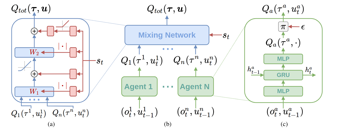
Figure 1: (a) Mixing network structure. In red are the hypernetworks that produce the weights and biases for mixing network layers shown in blue
The Agent Network consist of \(MLP + GRU + MLP\). Their input is the history of observation-action sequences of the respective agent, and their output is the decomposed Q-value function of that agent. The agent uses this Q-value to derive an \(\epsilon -greedy\) policy for exploration.
The Mixing Network takes two inputs: the outputs of all agent networks \(`\{Q_i(\tau^i,u_t^i)\}_{i=1}^N`\) and the global state \(`s_t`\) of the system. Its output is \(`Q_{tot}(\boldsymbol{\tau},\boldsymbol{u})`\). Notably, QMIX uses \(s_t\) as input to the Hypernetworks, which then generate parameters for the Mixing Network. This differs from VDN, which does not use the global state \(s_t\).
The key part of Figure 1 is the internal structure of the mixing network on the left. The Mixing Network includes an input layer, a hidden layer, and an output layer. Unlike a standard single-hidden-layer MLP, the weights and biases of its hidden layer are computed by another set of networks (Hypernetworks). The activation function for the hidden layer of the Mixing Network is ELU (Exponential Linear Unit), and the output layer uses linear activation (no activation function). As seen from the red block diagram:
\(W_1\) and \(W_2\) are generated by two single-layer linear networks followed by an absolute value activation.
The bias term corresponding to \(W_1\) is computed directly by a single-layer linear network (no activation).
The bias term corresponding to \(W_2\) is computed by a two-layer linear network, with the first layer using ReLU activation.
The Hypernetworks output a vector, which is then reshaped into the parameters of the Mixing Network.
You may wonder why the authors designed such an unusual structure to compute the Mixing Network’s parameters. In fact, this design ensures that the weight parameters of the mixing network are non-negative, allowing the Mixing Network to approximate any monotonic function (i.e., satisfying Equation\(`(3)`\)) with arbitrary precision.
To help readers better understand this logic, we expand the expression of the Mixing Network:
Here, \(Q=[Q_{1}(\tau^{1},u_{t}^{1}),\cdots,Q_{n}(\tau^{n},u_{t}^{n})]\) is an \(n\)-dimensional vector, and \(B_1\), \(B_2\) are the bias terms corresponding to \(W_1\), \(W_2\), respectively. Using the chain rule and the differentiation rule for linear transformations:
From the ELU activation function curve and its first derivative curve, we know that \(0<\frac{\partial\mathrm{Elu}(x)}{\partial x}\leq1\), Since every element in \(W_1\), \(W_2\) is non-negative, every element in \(\frac{\partial Q_{\mathrm{tot}}}{\partial \boldsymbol{Q}}\) (i.e., \(\frac{\partial Q_{\mathrm{tot}}}{\partial Q_i}\)) is also non-negative, so Equation \(`(3)`\) holds.
From the above analysis, we only need to ensure that the elements in weight matrices \(W_1\) and \(W_2\) are non-negative to achieve our goal —no restrictions are needed on the bias terms \(B_1\) or \(B_2\).
However, one might ask: Can a network constructed in this way serve as a universal function approximator?
The authors reference the conclusion from the following paper to answer this question: original paper link.
The paper shows that when the weight parameters of a neural network are restricted to be non-negative, it can theoretically approximate the following monotonic function with arbitrary precision \(\epsilon\):
Parameter Training
Since the input to all hypernetworks is the global state \(s_t\) and the output of the hypernetworks is the parameters of the Mixing Network, the parameters to be trained include Hypernetwork parameters and Agent Network parameters.
The authors use end-to-end training to minimize the following loss function:
where \(b\) is the batch size, \(y^{tot}=r+\gamma\max_{\boldsymbol{u}^{\prime}}Q_{tot}(\boldsymbol{\tau}^{\prime},\boldsymbol{u}^{\prime},s^{\prime};\theta^{-})\), and \(\theta^{-}\) denotes the target network parameters. The specific training process is similar to that of DQN.
Because the design of the mixing network ensures Equation\(`(1)`\) holds, solving \(\max_{\boldsymbol{u}^{\prime}}Q_{tot}(\boldsymbol{\tau}^{\prime},\boldsymbol{u}^{\prime},s^{\prime};\theta^{-})\) can be achieved by maximizing the value function of each agent individually. This greatly simplifies the computational complexity of solving the max function.
Function Representation Complexity
Although QMIX has stronger function fitting capability than VDN, the authors also note that the constraint in Equation\(`(3)`\) still limits the range of value functions it can fit. This is because some value function decompositions may not be based on satisfying this monotonicity constraint—Equation\(`(3)`\) is a sufficient but not necessary condition for Equation\(`(1)`\).
For some decentralized policies where the optimal action of a single agent depends on the actions of other agents at the same time, the function representation capability of the QMIX algorithm will also be limited to a certain extent. However, regardless, QMIX is still more powerful than VDN.
Conclusion
The QMIX algorithm has more advantages than VDN both in theory and experimental validation. As a value-based MARL algorithm, it is widely favored by researchers.
However, as noted by the authors, QMIX does not consider the actions of other agents when executing policies. This is somewhat unreasonable in practical scenarios. For multi-agent scenarios involving cooperative tasks, only by fully considering the potential impact of other agents on one’s own decisions can better cooperation be achieved. Therefore, considering more complex relationships between agents—such as task/role assignment and agent communication—is also an important direction for the extension of the QMIX algorithm.
Additionally, Equation\(`(3)`\) is a sufficient but not necessary condition for Equation\(`(1)`\), which limits the function approximation capability of the QMIX network to a certain extent. In some scenarios, this leads to a gap between the fitted \(Q_{tot}\) and the true value \(Q_{{tot}}^*\).
Run QMIX in XuanCe
Before running QMIX in XuanCe, you need to prepare a conda environment and install xuancefollowing
the installation steps.
Run Build-in Demos
After completing the installation, you can open a Python console and run QMIX directly using the following commands:
import xuance
runner = xuance.get_runner(algo='qmix',
                           env='mpe',  # Choices: football, mpe, sc2
                           env_id='simple_spread_v3',  # Choices: simple_spread_v3, etc
                           )
runner.run()
Run With Self-defined Configs
If you want to run QMIX with different configurations, you can build a new .yaml file, e.g., my_config.yaml.
Then, run the QMIX by the following code block:
import xuance as xp
runner = xp.get_runner(algo='qmix',
                       env='mpe',  # Choices: football, mpe, sc2
                       env_id='simple_spread_v3',  # Choices: simple_spread_v3, etc
                       config_path="my_config.yaml",  # The path of my_config.yaml file should be correct.
                       )
runner.run()  # Or runner.benchmark()
To learn more about the configurations, please visit the tutorial of configs.
Run With Custom Environment
If you would like to run XuanCe’s QMIX in your own environment that was not included in XuanCe,
you need to define the new environment following the steps in
New Environment Tutorial.
Then, prepapre the configuration file
qmix_myenv.yaml.
After that, you can run QMIX in your own environment with the following code:
import argparse
from xuance.common import load_yaml
from xuance.environment import REGISTRY_ENV
from xuance.environment import make_envs
from xuance.torch.agents import QMIX_Agents

configs_dict = load_yaml(file_dir="qmix_myenv.yaml")
configs = argparse.Namespace(**configs_dict)
REGISTRY_ENV[configs.env_name] = MyNewEnv

envs = make_envs(configs)  # Make parallel environments.
Agent = QMIX_Agents(config=configs, envs=envs)  # Create QMIX agents from XuanCe.
Agent.train(configs.running_steps // configs.parallels)  # Train the model for numerous steps.
Agent.save_model("final_train_model.pth")  # Save the model to model_dir.
Agent.finish()  # Finish the training.
Citation
@InProceedings{pmlr-v80-rashid18a,
  title={QMIX: Monotonic Value Function Factorisation for Deep Multi-Agent Reinforcement Learning},
  author={Rashid, Tabish and Samvelyan, Mikayel and Schroeder, Christian and Farquhar, Gregory and Foerster, Jakob and Whiteson, Shimon},
  booktitle={Proceedings of the 35th International Conference on Machine Learning},
  pages={4295--4304},
  year={2018},
  editor={Dy, Jennifer and Krause, Andreas},
  volume={80},
  series={Proceedings of Machine Learning Research},
  month={10--15 Jul},
  publisher={PMLR}
}
@article{rashid2020monotonic,
  title={Monotonic value function factorisation for deep multi-agent reinforcement learning},
  author={Rashid, Tabish and Samvelyan, Mikayel and De Witt, Christian Schroeder and Farquhar, Gregory and Foerster, Jakob and Whiteson, Shimon},
  journal={Journal of Machine Learning Research},
  volume={21},
  number={178},
  pages={1--51},
  year={2020}
}