Mean-Field Actor-Critic (MFAC)¶

Paper Link: https://proceedings.mlr.press/v80/yang18d/yang18d.pdf

Mean Field Actor-Critic (MFAC) is a crucial multi-agent reinforcement learning (MARL) algorithm that integrates the Actor-Critic framework. It introduces the “mean field approximation” to model the collective behavior of all agents, rather than explicitly considering the interaction between every pair of agents, thereby simplifying the learning process in large-scale multi-agent systems.

This table lists some general features about MFAC algorithm:

Features of MFAC	Values	Description
On-policy	✅	The evaluate policy is the same as the target policy.
Off-policy	❌	The evaluate policy is different from the target policy.
Model-free	✅	No need to prepare an environment dynamics model.
Model-based	❌	Need an environment model to train the policy.
Discrete Action	✅	Deal with discrete action space.
Continuous Action	✅	Deal with continuous action space.

Nash Q-learning¶

The Nash equilibrium is a core concept in game theory, referring to a stable state where no participant can improve their own payoff by unilaterally changing their strategy. In stochastic games, the Nash equilibrium is described as follows:

\[ v^j(s; \mathbf{\pi}_{*}) = v^j(s; \pi_{*}^j, \mathbf{\pi}_{*}^{-j}) \geq v^j(s; \pi^j, \mathbf{\pi}_{*}^{-j}) \]

Here,$s$ is the state,$\pi_*$ is all agents adopt the equilibrium strategy(where $\pi_*^{j}$ the equilibrium strategy of agent $j$ and $\pi_*^{-j}$ is the equilibrium strategy profile of all agents except ${j}$),$v^{j}(s,\pi_*)$ is the value of agent $j$. This formula can be understood as: No agent can increase its own value in the current state by unilaterally changing its strategy.

In a Nash equilibrium,give a Nash policy $\pi_*$,the Nash value function $\mathbf{v}^{nash}(s)\triangleq[v^{1}_{\pi_*}(s),\dots,v^{N}_{\pi_*}(s)]$, the Nash value function represent the Q function:

\[ \mathcal{H}^{\text{Nash}} \mathbf{Q}(s, \mathbf{a}) = \mathbb{E}_{s' \sim p} \left[ \mathbf{r}(s, \mathbf{a}) + \gamma \mathbf{v}^{\text{Nash}}(s') \right] \]

Here,$\begin{cases} \mathbf{Q} \triangleq [Q^1, \dots, Q^N], \\ \mathbf{r}(s, \mathbf{a}) \triangleq [r^1(s, \mathbf{a}), \dots, r^N(s, \mathbf{a})]\end{cases}$

Mean Field MARL¶

The dimension of the joint action space grows proportionally with respect to the number of agents $N$.To address this issue, The Q-function is factorized by leveraging only pairwise local interactions:

\[ Q^{j}(s, \mathbf{a}) = \frac{1}{N^{j}} \sum_{k \in \mathcal{N}(j)} Q^{j}(s, a^{j}, a^{k}) \]

Where $\mathcal{N}(j)$ is the index set of the neighboring agens of agent $j$ with the size $N(j)=|\mathcal{N}(j)|$ determined by the settings of different applications.

Mean Field Approximation¶

Compute the second-order Taylor derivative for $Q^{j}(s, \mathbf{a})$ with respect to the action $a_k=\bar{a}^j$:

\[\begin{split} \begin{aligned} Q^j(s,\mathbf{a}) = \frac{1}{N^j} \sum_k Q^j(s, a^j, a^k) \\ & = \frac{1}{N^j} \sum_k \left[ Q^j(s, a^j, \bar{a}^j) + \nabla_{\bar{a}^j} Q^j(s, a^j, \bar{a}^j) \cdot \delta a^{j,k} + \frac{1}{2} \delta a^{j,k} \cdot \nabla_{ \tilde{a}^{j,k}}^2 Q^j(s, a^j, \tilde{a}^{j,k}) \cdot \delta a^{j,k} \right] \\ & = Q^j(s, a^j, \bar{a}^j) + \nabla_{\bar{a}^j} Q^j(s, a^j, \bar{a}^j) \cdot \left[ \frac{1}{N^j} \sum_k \delta a^{j,k} \right] + \frac{1}{2N^j} \sum_k \left[ \delta a^{j,k} \cdot \nabla_{\tilde{a}^{j,k}}^2 Q^j(s, a^j, \tilde{a}^{j,k}) \cdot \delta a^{j,k} \right] \\ & = Q^j(s, a^j, \bar{a}^j) + \frac{1}{2N^j} \sum_k R^j_{s,a^j}(a^k) \approx Q^j(s, a^j, \bar{a}^j) \end{aligned} \end{split}\]

Where,$\sum_k R^j_{s,a^j}(a^k) \triangleq \sum_k \left[ \delta a^{j,k} \cdot \nabla_{\tilde{a}^{j,k}}^2 Q^j(s, a^j, \tilde{a}^{j,k}) \cdot \delta a^{j,k} \right] $ denotes the Taylor polynomial’s remainder with $\tilde{a}^{j,k} = \bar{a}^{j} + \epsilon^{j,k} \delta a^{j,k}$, $\epsilon^{j,k} \in [0,1]$. Here, Represent $a^j$ using one-hot encoding: $a^j \triangleq [a_1^j, \dots, a_N^j]$, $\bar{a}^j$ is the mean action of the agent’s neighbors $\mathcal{N}(j)$. The action $a_k$ of each neighbor is expressed as the sum of $\bar{a}^j$ and a small fluctuation $\delta a^{j,k}$:

\[ a^k = \bar{a}^j + \delta a^{j,k}, \quad \text{where} \ \bar{a}^j = \frac{1}{N^j} \sum_k a^k \]

Thus, Many agent interactions are effectively converted into two agent interactions, $Q^j(s,\mathbf{a})\approx Q^j(s, a^j, \bar{a}^j)$. Developing practical mean field Q-learning and mean field Actor-Critic algorithms.

Iteration Of Q-function¶

MFAC algorithm updates the Q-function through Temporal Difference (TD) learning, whose core idea is to “correct the current Q-value using the currently estimated future Q-value”. At this point, given an experience $e = (s, \{a^{k}\}, \{r^{j}\}, s')$ the update function of the mean field Q-function is:

\[ Q_{t+1}^j(s, a^j, \bar{a}^j) = (1 - \alpha) Q_t^j(s, a^j, \bar{a}^j) + \alpha \left[ r^j + \gamma v^j_t(s') \right] \]

Where $\alpha$ is the learning rate, $\gamma$ is the discount factor, the mean field value function $ v^j(s')$ is:

\[ v_t^j(s') = \sum_{a^j} \pi^j_t(a^j | s', \bar{a}^j) \mathbb{E}_{\bar{a}^j(\mathbf{a}^{-j}) \sim \ \mathbf{\pi}^{-j}} \left[ Q_t^j(s', a^j,\bar{a}^j) \right] \]

To distinguish from the Nash value function $\mathbf{v}^{\text{Nash}}(s)$, the above formula as $\mathbf{v}^{\text{MF}}(s)\triangleq[v^1(s),\dots,v^N(s)]$. Defining the mean field operator $\mathcal{H}^{\text{MF}}:\mathcal{H}^{\text{MF}}\mathbf{Q}(s, \mathbf{a}) = \mathbb{E}_{s' \sim p} \left[ \mathbf{r}(s, \mathbf{a}) + \gamma \mathbf{v}^{\text{MF}}(s') \right]$. In fact, when $\mathcal{H}^{\text{MF}}$ forms a contraction mapping, that is, one updates $\mathbf{Q}$ by iteratively applying the mean field operator $\mathcal{H}^{\text{MF}}$, the mean field Q-function will eventually converge to the Nash Q-value under certain assumptions. (Specific assumptions and convergence proofs can be found in the paper.)

Main Idea¶

MFAC adopts the Actor-Critic (AC) framework. Actor Critic Method selects actions through the Actor, evaluates these actions through the Critic, and cooperates with each other to improve.

Compare With MFQ¶

Just like MFQ, MFAC also draws on the stable training techniques of DQN in deep reinforcement learning, and adopts the ideas of experience replay and target network. However, in terms of policy update, MFAC explicitly models the policy using neural networks with weights $\theta$.

Update Critic¶

Critic is also called value network, just like MFQ updates its $Q$ network, MFAC also achieves this through the following steps.

sampling experience: Sample minibatch experiences $(s, \mathbf{a}, \mathbf{r}, s', \mathbf{\bar{a}})$ from the experience replay buffer $\mathcal{D}$
Inherited Average Action: Sample the action $a^j_-$ from the target network $Q_{\phi^j_-}$, and let the target network inherit the current average action estimation.

In MFAC, agent $j$ is trained by minimizing the loss function:

\[ \mathcal{L}(\phi^j) = \left( y^j - Q_{\phi^j}(s, a^j, \bar{a}^j) \right)^2 \]

Where $y^j = r^j + \gamma v_{\phi^j_-}^{\text{MF}}(s')$, and $\phi^j_-$ is the parameters of the target network.

Finally, Don’t forget update the parameters of the target $Q$ network:

\[ \phi^j_- \leftarrow \tau_\phi \phi^j + (1 - \tau_\phi) \phi_-^{j} \]

Here, $\tau_\phi$ is learning rate.

Update Actor¶

{% raw %} Actor is also called policy network, for each agent $j$, MFAC provides current policy network $\pi_{\theta^{j}}$ and target policy network $\pi_{{\theta^{j}}_\_}$, $\theta^j$ and ${\theta^{j}}_\_$ are parameters. {% endraw %}

Under state $s$, agent $j$’s action $a^j=\pi_{\theta^{j}}(s)$, new mean action $\mathbf{\bar{a}}$ = $[\bar{a}^1, \dots, \bar{a}^N]$ and the calculation formula:

\[ \bar{a}^j = \frac{1}{N^j} \sum_k a^k, a^k \sim \pi_t^k(\cdot |s,{\bar{a}^k}_\_) \]

Here, agent $j’s$ $N_j$ neighbors from the policies $\pi^k_t$ parametrized by their previous mean actions ${\bar{a}^k}_\_$. Just like MFQ, store the experience tuple $(s, \mathbf{a}, \mathbf{r}, s', \mathbf{\bar{a}})$ in the experience replay buffer $\mathcal{D}$.

Update the actor using the sampled policy gradient:

{% raw %} $$ \nabla_{\theta^j} \mathcal{J}(\theta^j) \approx \sum \left. \nabla_{\theta^j} \log \pi_{\theta^j}(s') Q_{\phi^j_-}(s', {a^j}_\_, {\bar{a}^j}_\_) \right|_{{a^j}_\_ = {\pi_{\theta^j}}_\_(s')} $$ {% endraw %}

Finally, Don’t forget update the parameters of the target policy network:

\[ \theta^j_- \leftarrow \tau_\theta \theta^j + (1 - \tau_\theta) \theta_-^{j} \]

Here, $\tau_\theta$ is learning rate.

Strengths of MFAC:

The algorithm adopts Actor-Critic as its framework. It can not only quickly locate effective actions but also accurately optimize the policy.
The algorithm employs mean field theory, using the “mean value of the collective actions” to approximate the influence of other agents on the current agent, thereby solving the problem of state space explosion in multi-agent scenarios.
Draw on the stable training techniques of DQN, such as experience replay and target network.

Algorithm¶

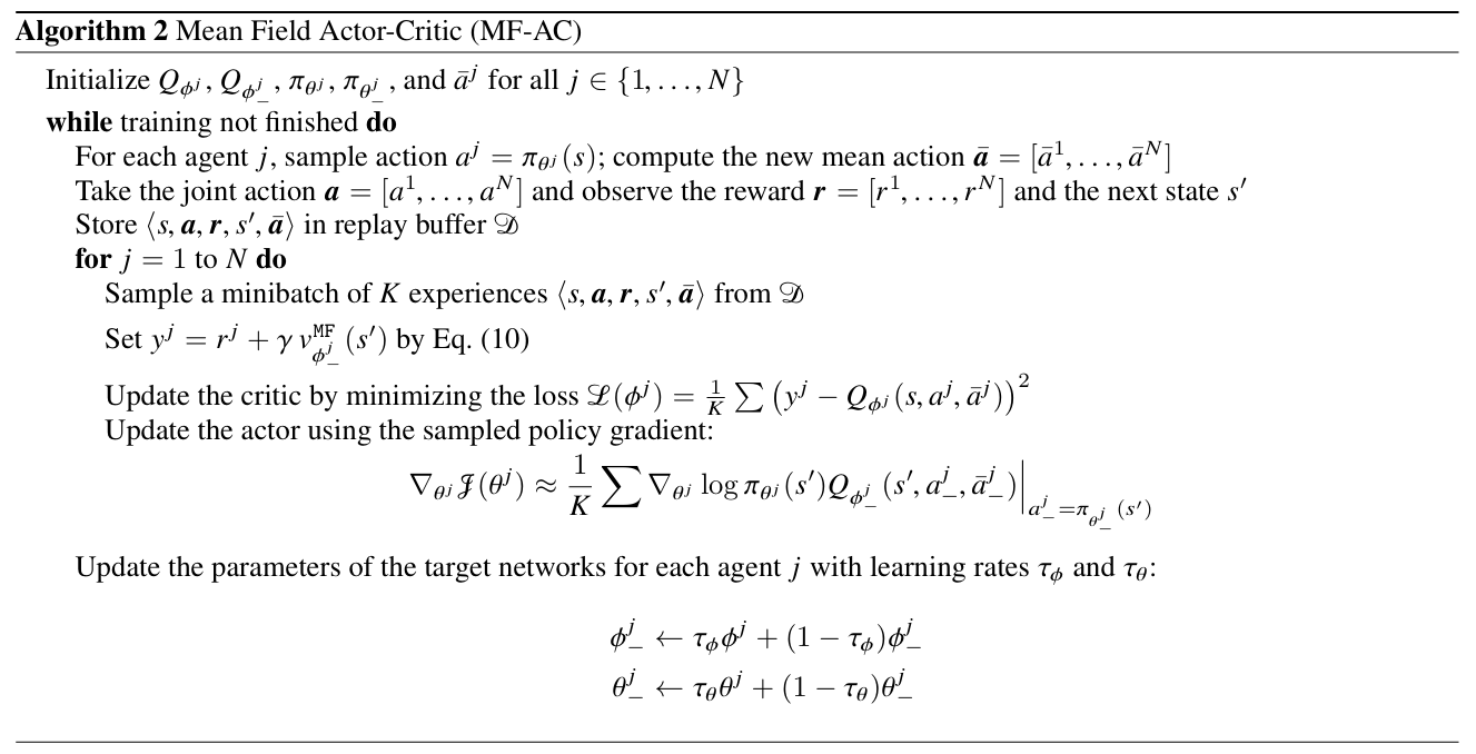
The full algorithm for training MFAC is presented in Algorithm 2:

Run MFAC in XuanCe¶

Before running MFAC in XuanCe, you need to prepare a conda environment and install xuance following the installation steps.

Run Build-in Demos¶

After completing the installation, you can open a Python console and run MFAC directly using the following commands:

import xuance
runner = xuance.get_runner(algo='mfac',
                           env='classic_control',  # Choices: claasi_control, box2d, atari.
                           env_id='CartPole-v1',  # Choices: CartPole-v1, LunarLander-v3, ALE/Breakout-v5, etc.
                           )
runner.run()  # Or runner.benchmark()

To learn more about the configurations, please visit the tutorial of configs.

Run With Custom Environment¶

If you would like to run XuanCe’s MFAC in your own environment that was not included in XuanCe, you need to define the new environment following the steps in New Environment Tutorial. Then, prepapre the configuration file mfac_myenv.yaml.

After that, you can run MFAC in your own environment with the following code:

import argparse
from xuance.common import load_yaml
from xuance.environment import REGISTRY_ENV
from xuance.environment import make_envs
from xuance.torch.agents import MFAC_Agent

configs_dict = load_yaml(file_dir="mfac_myenv.yaml")
configs = argparse.Namespace(**configs_dict)
REGISTRY_ENV[configs.env_name] = MyNewEnv

envs = make_envs(configs)  # Make parallel environments.
Agent = MFAC_Agent(config=configs, envs=envs)  # Create a MFAC agent from XuanCe.
Agent.train(configs.running_steps // configs.parallels)  # Train the model for numerous steps.
Agent.save_model("final_train_model.pth")  # Save the model to model_dir.
Agent.finish()  # Finish the training.

Citation¶

@InProceedings{pmlr-v80-yang18d,
  title = 	 {Mean Field Multi-Agent Reinforcement Learning},
  author = 	 {Yang, Yaodong and Luo, Rui and Li, Minne and Zhou, Ming and Zhang, Weinan and Wang, Jun},
  booktitle = 	 {Proceedings of the 35th International Conference on Machine Learning},
  pages = 	 {5571-5580},
  year = 	 {2018},
  editor = 	 {Dy, Jennifer and Krause, Andreas.},
  volume = 	 {80},
  series = 	 {International Conference on Machine Learning},
  address = 	 {Stockholmsmässan, Stockholm Sweden},
  month = 	 {10--15 July},
  publisher =    {PMLR},
  pdf = 	 {https://proceedings.mlr.press/v80/yang18d/yang18d.pdf},
  url = 	 {https://proceedings.mlr.press/v80/yang18d.html},
  abstract = 	 {Existing multi-agent reinforcement learning methods are limited typically to a small number of agents. When the agent number increases largely, the learning becomes intractable due to the curse of the dimensionality and the exponential growth of agent interactions. In this paper, we present Mean Field Reinforcement Learning where the interactions within the population of agents are approximated by those between a single agent and the average effect from the overall population or neighboring agents; the interplay between the two entities is mutually reinforced: the learning of the individual agent’s optimal policy depends on the dynamics of the population, while the dynamics of the population change according to the collective patterns of the individual policies. We develop practical mean field Q-learning and mean field Actor-Critic algorithms and analyze the convergence of the solution to Nash equilibrium. Experiments on Gaussian squeeze, Ising model, and battle games justify the learning effectiveness of our mean field approaches. In addition, we report the first result to solve the Ising model via model-free reinforcement learning methods.}
}